Lessons from the Quant Winter

The quant winter was a two‑year period from 2018 to 2020 when quant funds underperformed. This was largely a Developed Markets effect, with Australia also affected, and Emerging Markets showed a different profile (shorter and sharper).

The main culprit was Value, which performed poorly (and progressively worse) as the period went on. Other factors like Growth and Momentum – which usually compensate for Value underperformance – and Low Volatility did not. Quality performed relatively well.

The “why” is not clear. Low inflation and the growth of big tech from about 2015 are certainly contributors, but the lack of performance of Growth and Momentum is still a puzzle.

By using a perfect forecast or “oracle” approach, we see that it would have been difficult to position a quant factor model any differently.

The last few years have shown strong quant factor performance and have raised questions of whether a quant winter could recur. We believe this period is more of a recovery from the winter than a precursor to another factor drought.

The so‑called “quant winter”¹ of 2018 to 2020 was a watershed for quant investors and their clients. Quant funds had advertised (and delivered) consistent performance above benchmarks for some time, even for more generic factors like simple value ratios and price momentum.

Starting around the beginning of 2018, this consistent performance began to unwind. Nomura, in a private research note, found that only 15% of quant funds beat their benchmarks in 2018 and 2019.²

This underperformance was so severe and extended that many clients abandoned quant, quant funds lost large amounts of FUM and staff,³ and even seasoned sell side analysts “gave up”.⁴

In early 2020, Covid‑19 took over and the world will never be the same, as we know. This led to many dramatic changes to the business and investment landscape. Among them, quant factors started working again and have generally been strong ever since. All, it seems, is forgiven.⁵

Or is it? Many still question the validity of this recent bounce back, concentration of quant factors and the likelihood of another quant winter. It is too close in recent memory to be assigned to history like other dislocations: the GFC of 2007 to 2009 or the tech meltdown of 2000.

While we cannot (in fact no‑one can) answer the question of when or if another quant winter might occur, we can throw some light on some questions: what it was, what might have caused it, and whether or not it could have been avoided. For this last question we use what we call “oracle” or perfect foresight analysis, which allows us to see whether we could have done anything differently if we had known in advance of this period of poor quant factor performance. As we note in more detail later, a first‑rate oracle would be able to predict exactly which stocks will outperform. Our “second‑rate” oracle can only tell us in which quintile of returns a stock will belong.

What was the Quant Winter?

What has become known as the quant winter was a period of a little over two years, from early 2018 to mid‑2020. It was characterised by consistent poor performance of quant funds against their benchmarks.

Chart 1 below is from a private Nomura research paper, via the FT.⁶ It shows that in 2018 and 2019 only about 15% of quant funds outperformed, while in 2017 it was above 60%.

Chart 1: Percentage of outperforming quant funds by year

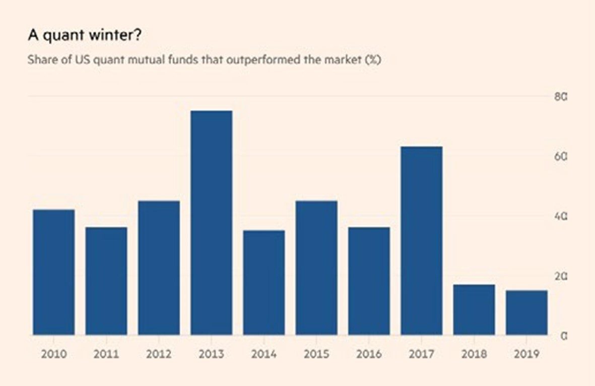
Source: Nomura, 2020

This is especially disturbing as quant funds are considered (and indeed market themselves) as being consistent alpha sources throughout economic cycles – that is, as various economic drivers impact different sources of alpha. Quant funds will usually – but not always – have a diversified mix of expected return drivers (alpha sources) and in history it is very unusual for all of them to stop or misfire at the same time.⁷

We will not explore all of our quant factors and their performance during this period. Instead, we will restrict ourselves to those of most interest. In particular, we will look at Value (proxied by 12 month forward earnings yield, or EY_NTM), Momentum (proxied by 12‑month return less the most recent month), Volatility (proxied by last 12 months daily volatility), Quality (proxied by return on equity or ROE) and Growth (proxied by expected EPS growth to the next end of financial year).⁸

Data is from the MSCI World ex Australia universe.

In summary, we find that Value was the main culprit. Being long Value (holding cheaper names) was costly throughout this period and indeed became progressively worse over time. We also found that exposure to low volatility paid off early in the sample period but was costly later.

In an environment where Value underperforms, we have commonly seen a rotation to Momentum or Growth. That is, Value tends to have low correlation with these two factors. However, we did not see any benefit from being long Momentum or Growth during this period – our oracle shows this.

If Value is underperforming, there are two intertwined reasons. Either the market is paying up excessively for earnings growth, or valuation multiples are expanding – or both. We see that earnings growth did not pay off during the quant winter, which means that Value’s underperformance was due to the market paying more for the same earnings.

Finally, we see that a Quality (ROE) tilt did have a positive return, so we further ask the question of whether portfolios which combined Quality with Value would have done better than those which concentrated on Value alone. We find that this is not the case – expensive quality outperformed cheap quality.

Chart 2 Panel A on the next page shows the returns to quintiles of value from Jan 1 2017 to Jan 1 2021. We use EY_NTM as our value measure. That is, at each date we sort all stocks into quintiles from Low (most expensive) to High (cheapest) stocks based on EY_NTM. We then calculate the mean return for each quintile and calculate the cumulative return over the period.⁹

Chart 2 Panel A: Performance of Value quintiles (measured as EY_NTM)

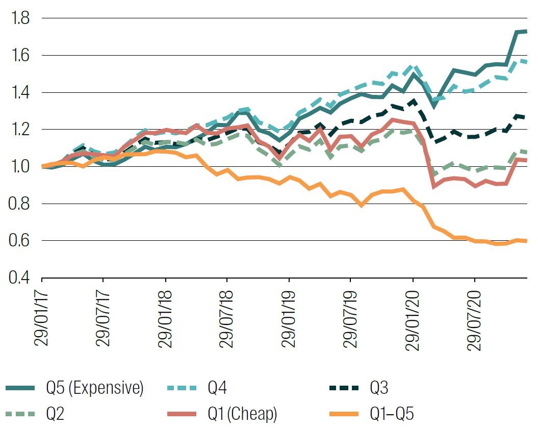
1 Jan 2017 to 1 Jan 2021.
Source: RQI Investors, MSCI, 2025.

The dark green line in Chart 2 is the cumulative return for the most expensive quintile of stocks, and the red line is the cumulative return for the cheapest quintile. If investing in Value was paying off, the red line would trend upwards and the dark green line would trend downwards.

We see exactly the opposite to this, starting from early 2018, although the most dramatic moves happened early in 2019. Returns to the most expensive stocks significantly outperformed the cheapest until the beginning of 2021. To reinforce this, the orange line is the difference in return between Q1 (cheapest) and Q5 (most expensive). It starts mildly positive until early 2018 and then trends down sharply.

Chart 2 Panel B then extends the sample period out to the end of April 2025. We can see clearly that following this Value underperformance period (the “quant winter” period), the most expensive stocks sold off sharply and the cheapest stocks rebounded, delivering the strong performance to Value from early 2021 until recently.

Note that cheapest names rebounded (point B) well before the expensive stocks sold off (point A) so the quant winter period was shortened somewhat, and managers were cushioned from the strongest performance of the most expensive stocks from mid‑2020 until mid‑2021.

Chart 2 Panel B: Performance of Value quintiles (measured as EY_NTM)

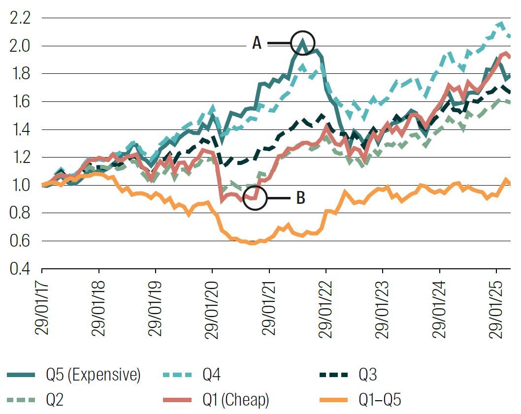
1 Jan 2017 to 1 May 2025.
Source: RQI Investors, MSCI, 2025.

Chart 3 shows the payoffs to momentum and quality over the same period as Chart 2 Panel A, where each quintile’s return is charted cumulatively. While momentum was slightly positive over the period of the quant winter (high momentum outperforms low momentum) the spread is not large – certainly not enough to compensate for the underperformance of value, if the two were combined. Following this period, momentum (and value as we saw earlier) performed very well.

Note: Momentum underperformed slightly in early 2018 at the same time as Value, but then as Value’s underperformance worsened, Momentum became flat and then went positive in advance of the eventual return of Value to positive performance.

Chart 3 Panel A: Performance of Momentum quintiles (measured as 12-month return less most recent 1 month)

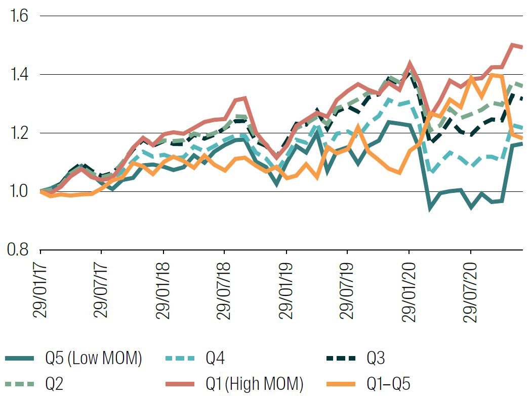
1 Jan 2017 to 1 Jan 2021.
Source: RQI Investors, MSCI, 2025.

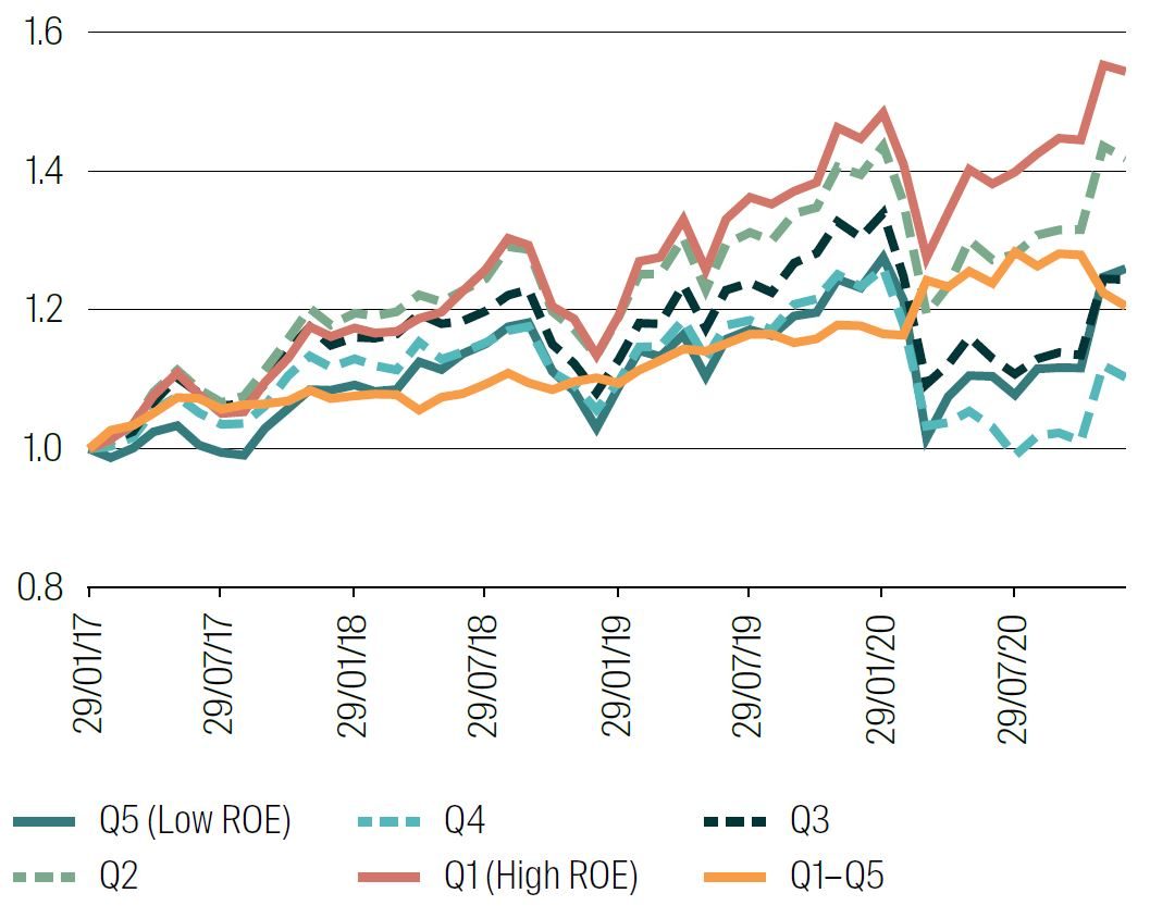
Quality is a different story. Good quality stocks (Q1) mildly outperformed poor‑quality stocks (Q5) during the start of the quant winter, and then strongly outperformed towards the end and later into the Covid‑19 period.

Chart 3 Panel B: Performance of Quality quintiles (measured as ROE)

1 Jan 2017 to 1 Jan 2021.
Source: RQI Investors, MSCI, 2025.

Potential causes?

Isolating a single cause of the quant winter is probably impossible. At first blush there are a number of possible explanations which, in combination, led to this period of factor underperformance. Here we select six of the likely culprits, and with each we will assess the weight each might have had in driving this period. Each in isolation can be suggested as a contributor, although they overlap and some can be dismissed.

Growth and valuation multiple expansion of big US tech

In our opinion, this is the main driver of the underperformance of Value during this period. The growth in the largest stocks in the US has been dramatic since about 2015, as we saw in our recent paper on Market Concentration.¹⁰

Chart 7 from that paper shows that the weight of the top 10 names in MSCI World steadily increased from about 10% in 2015 to more than 25% by late 2024. From 20170101 to 20210101 (the quant winter period), the growth was from 11% to 19%.

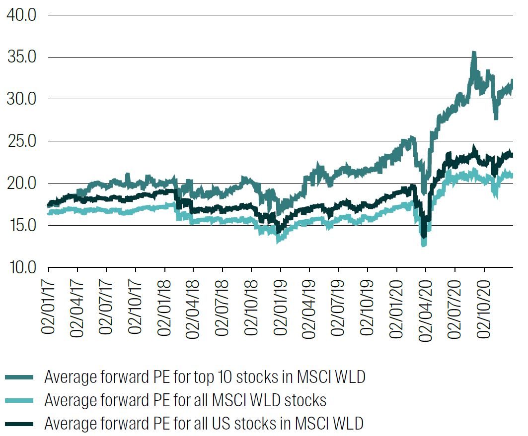
These stocks trade at much higher multiples than the market, and this spread widened very sharply, from late 2018. Chart 4 below shows the average 12‑month forward PE ratio for MSCI World, for just the US stocks in MSCI World, and for just the top 10 stocks in MSCI World.

Chart 4: Forward PE multiples over the quant winter period

Source: RQI Investors, MSCI, 2025.

Crowding of factors or increased correlation through quant fund growth

This idea is often resurrected as a likely cause of any quant fund issues. Certainly, factor crowding has been a problem in the past, with the GFC being the prime example. There we found that many quant fund returns were very correlated and negative when the market sold off.

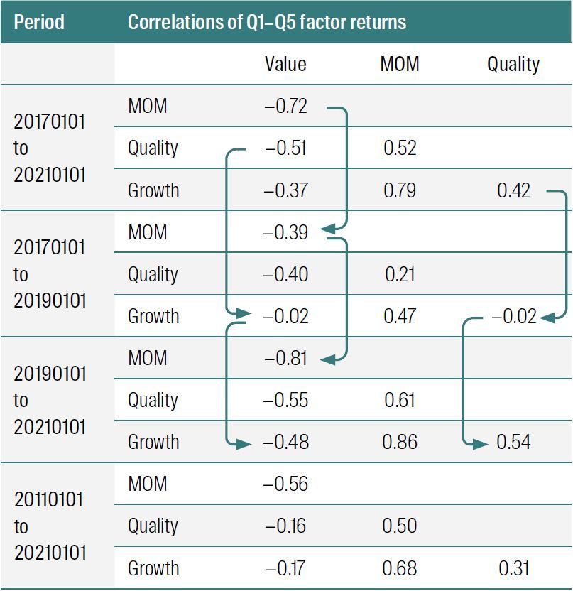
We do not think this is the case here. To begin, the change in the market was an acceleration of the growth of expensive US tech, which many quant funds would not own as overweight positions (expensive but yet to deliver growth). Further correlations between factors were very different across time periods, as Table 1 below shows. It is not increasing as crowding would suggest, although we do see VALUE becoming much less negatively correlated with MOM and GROWTH at the start of the quant winter but then reverting. QUALITY and GROWTH correlation also varies sharply over the period, although is positive overall.

Table 1: Correlation between Q1‑Q5 returns for VALUE (EY_NTM), MOM (12 month return less 1 month return), QUALITY (ROE) and GROWTH (forecast earnings change to next FY end), over various windows.

Source: RQI Investors, MSCI, 2025.

Academic data mining/overfitting

The problem of in‑sample testing versus out‑of‑sample performance is a topic of considerable interest to quant equity managers, especially those who follow academic publications closely. McLean and Pontiff (2016)¹¹ among others have explored the effect that many academic finance papers appear to show strong results for “anomalies” which then fail to perform post publication. This could be due to (a) overfitting in sample, (b) public release of the concept immediately prices it out or (c) the research itself faces a replication issue (like many other fields), where published results cannot be replicated reliably.¹²

Do quant funds adopt these newly released or published alpha sources directly into their models? If so, the disappearance of realised performance could relate to this. However, most quant managers (certainly those who are serious!) would not simply fold newly published ideas into their process without extensive testing and validation, taking the potential of overfitting into account. We certainly would not.

There are two other reasons to consider which reject this notion. Firstly, it is the behaviour of more standard or generic factors that seem to be at the heart of the quant winter. We have not examined more idiosyncratic (recently published) ideas because we have not needed to.

Secondly, as we noted above, the behaviour of these factors is not uniform, and so does not point to a central all‑encompassing factor driver like research overfitting. An explanation based on the impact it has had on the central factor of interest – Value – is much more sensible.

Low interest rates and inflation

Characteristics of the approximately 10 years between the GFC and Covid were low interest rates and low inflation. Policy decisions to help stimulate the economy and smooth the turbulence post‑GFC (like “quantitative easing”) were the main drivers. If a recession is “natural” following a period of excess,¹³ then these policies impeded that correction and effectively deferred or even quashed the fallout of the GFC (at least to the large banks).¹⁴

We already know that this led to a period which provided strong support for Growth as a style, evidenced by the underperformance of the Value style for most of that period.¹⁵ In some ways, this government or political policy encouraged a type of Growth bubble and supported the dramatic emergence of the tech giants.

On their own, low interest rates and inflation have provided the well‑known headwind to Value for most of the decade from 2011 but would not explain the sharp sell‑off from 2018. However, in combination with the growth in big tech the argument becomes much stronger.

The short side of a quant signal (in the case of Value) requires a reversion – where overconfidence is penalised when expected growth is not delivered. As we have already noted, the ongoing growth of big tech was a key driver of the quant winter, has not (yet) been penalised, and government policies provided much of that support.

Natural cyclicality in quant factors?

Do quant factors naturally exhibit cyclicality, and does this explain much off the quant winter? It is hard to argue against the idea that different types of quant factors work at different stages of the economic cycle. For example, for simple/generic factors:

• Quality factors tend to work well in economic downturns, Growth does not.
• Value factors work well in normal economic conditions when investors overestimate growth and oversell less glamorous stocks.
• Momentum works well in long‑term trending markets and very badly at market corners (that is, risk‑on or risk‑off).
• Growth works well in stimulatory low‑interest‑rate environments when multiples expand and earnings growth off a low base is actually delivered.
• Quality works poorly and deep Value works very well in the recovery phase following a downturn.

There are also examples of “seasonality” rather than cyclicality. Momentum in Australia tends to work especially well in June and then badly in July, due to tax loss selling and then repurchase.

To call these cycles in the sense that they are predictable or even recognisable in advance is a long bow to draw. In hindsight, we can usually identify them, and in the case of the quant winter we might reasonably have expected Value to underperform given interest rates and inflation were so low. What was probably impossible to predict using quant factors, and what seemed to drive most of the underperformance, was the emergence of new technologies and the seismic shift in the economy and markets it generated.

So, in answer to our question, there is probably detectable quant behaviour attached to certain market regimes, with hindsight, but contribution to the quant winter was probably muted.

¹ Attributed to both Cliff Asness at AQR and Joseph Mezrich at Nomura. At RQI, we find this term misleading, as if there might also be a quant spring, summer and autumn.

² See for example https://www.ft.com/content/8666e64a‑357f‑11ea‑a6d3‑9a26f8c3cba4.

³ See the well‑named FT article “A quant winter’s tale” https://www.ft.com/content/e0f98278‑432e‑4ece‑b170‑2c40e40d2835.

⁴ Not quite – see I. Fraser‑Jenkins, Alliance Bernstein research note “Why I am no longer a quant” from October 2020. What he is saying is that the quant world has changed and can no longer rely just on backtests and diversification. A more holistic approach to research and portfolio construction is required. We at RQI agree.

⁵ https://www.man.com/insights/the‑quant‑renaissance.

⁶ https://www.ft.com/content/8666e64a‑357f‑11ea‑a6d3‑9a26f8c3cba4.

⁷ For example, see https://investmentmoats.com/notes/notes‑quant‑winter‑robin‑wigglesworth/.

⁸ We have deliberately avoided looking at idiosyncratic quant factors and concentrated more on the generic. This is for two reasons – IP protection, and noting that idiosyncratic factors should be somewhat different for each manager.

⁹ By convention, Q1 is the “best” (best value, highest quality, …) and Q5 is the worst.

¹⁰ Walsh, D, RQI Investors, 2025, Extreme concentration and its implications for equity investors.
https://www.firstsentierinvestors.com.au/au/en/institutional/ insights/latest‑insights/extreme‑concentration‑and‑its‑implications‑for‑equity‑investors.html.

¹¹ McLean, R. David, and Jeffrey Pontiff, 2016, Does academic research destroy stock return predictability? Journal of Finance 71, 5–32.

¹² But see Jensen et al, 2023 “Is there a Replication Crisis in Finance?”, Journal of Finance, 78, 2465‑2518.

¹³ Best described as “creative destruction”.

¹⁴ Again see I. Fraser‑Jenkins, Alliance Bernstein research note “Why I am no longer a quant” from October 2020.

¹⁵ Artificially low interest rates provide a stimulus for Growth as long dated cash flows are inflated in Present Value calculations.

In the first chapter of this set, we looked at the period that constituted the so‑called “quant winter.” We examined the performance of selected factors and reached the conclusion that the main culprit was the Value Factor, compounded by a lack of response from Momentum or Growth. The dramatic growth of expensive US tech, initially from 2015 but then accelerating through to 2021 and beyond, was a strong contributor, firstly in line with earnings growth and then with dramatic PE multiple expansion.

We now move to ask – how should we have been positioned if we wanted to avoid underperformance during this period? The simple answer – don’t invest in Value – is not useful as every quant model worth its salt will include some set of value factors.¹

A better way to address this is see how we would have been positioned if we had some knowledge of the future. In other words, if we have access to an oracle, who could tell us what was about to happen, how would we act? What would pay off?

To make this useful, we must restrict this oracle in some way, or else we would be told either which stock would perform the best (in which case, just buy that stock) or which factor is the best (in which case we just use a quant model with this single factor). Neither of these throw much light on the question.

We propose a second‑rate oracle, rather than the first‑rate all‑seeing oracle above. This second‑rate oracle can only tell us in which quintile of future returns a stock belongs today.

For example, by visiting our second‑rate oracle we will get to know today if stock ABC will be in the top quintile of returns in (say) 12 months’ time. Our obvious investment strategy is then to go long quintile 1 and short quintile 5².

This is not insightful for our current question. More useful, perhaps, is to ask the question – what are the characteristics of the stocks in these quintiles? This helps us pose the entirely hypothetical question – how would we be positioned (that is, what factor exposures would we have) to capture this Q1–Q5 return spread?³

We restrict ourselves to a standard set of factors rather than searching for more idiosyncratic or esoteric factors that might have worked. That is not the intent of the exercise. Instead, we think of the more generic factors: Value, Volatility, Momentum, Quality and Growth.

Our universe is again MSCI World ex Australia.

To quantify the return side of this analysis, Chart 5 below shows the cumulative return to each quintile from 20170101 for 250 days. In detail:

We visit our oracle and get a stock list which – for each stock – tells us to which quintile of returns it belongs in 250 days’ time.

We buy a cap‑weighted portfolio of the stocks in each quintile today and then hold them for 250 days.⁴

We calculate the return to each quintile over that time.

Chart 5: Cumulative returns to oracle quintile portfolios – 250 days from Jan 1 2017

Source: RQI Investors, MSCI, 2025.

The difference is very large. The cumulative return spread Q1–Q5 is about 65% in one year. This is typical of most years in our sample.

Now, what are the characteristics of the stocks in each quintile? We start with Value (as EY_NTM). Chart 6 Panels A and B show the average Value exposure for each quintile and how is moves over time, plus the Q1‑Q5 Value spread. These charts are smoothed (equally weighted) averages over short‑ and long‑term windows (25 day and 250 day) to help interpretation.

Chart 6 Panels A and B: Value exposure in oracle quintiles
Average EY_NTM exposure in each quintile of future returns over the next 250 days

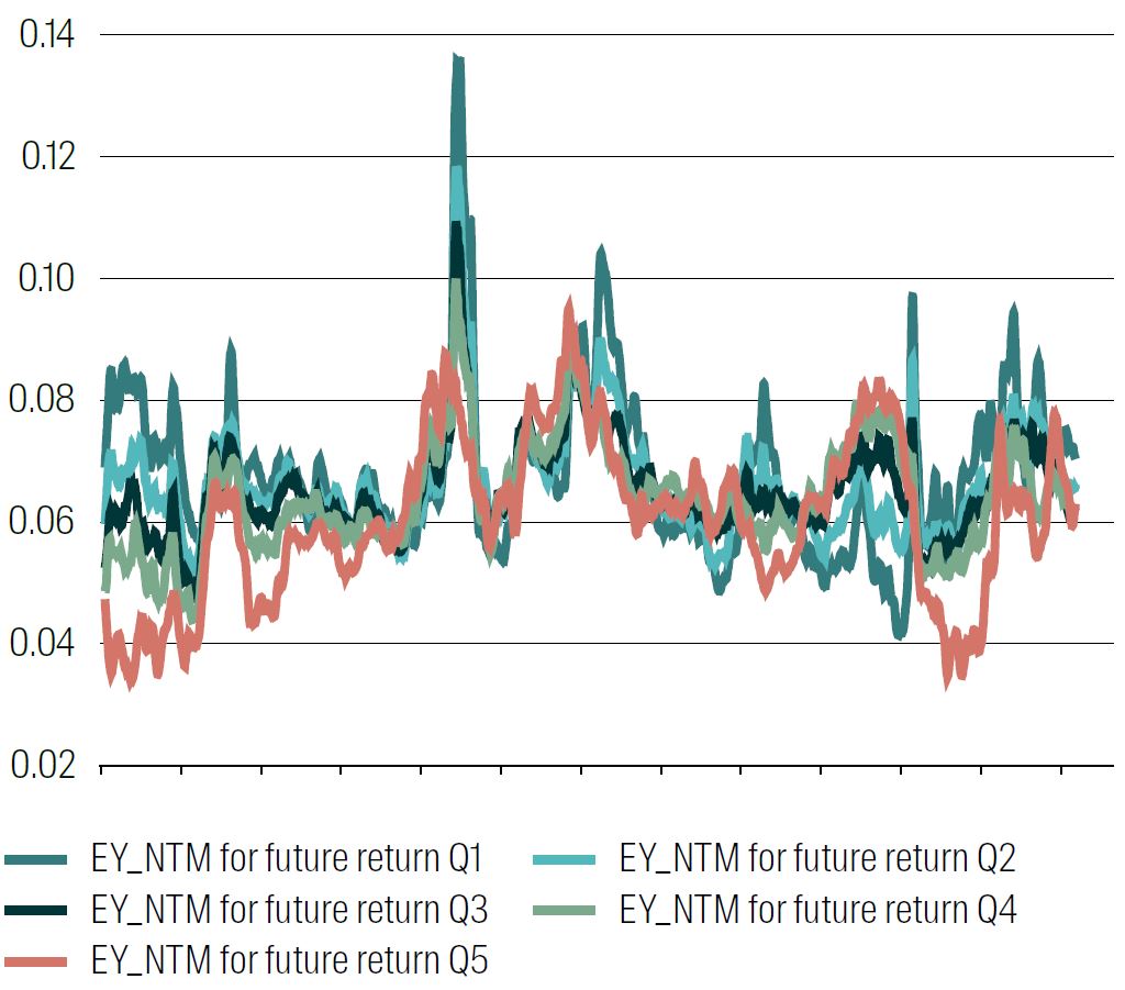
Q1 to Q5 spread exposure for EY_NTM over the next 250 days. (Negative means shorting the factor)

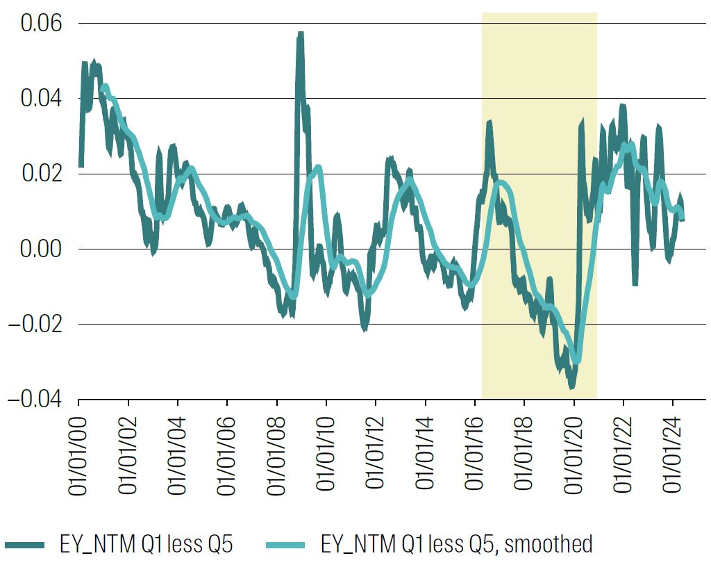
1 Jan 2000 to 1 Jan 2025.
Smoothing is via 25 day and 250 day rolling averages. Quant winter period is highlighted.

For most of the long sample period, it paid to be long cheap stocks (high EY_NTM) and short expensive stocks (low EY_NTM). There are short periods where it pays to bet on expensive stocks (spread exposure below zero) but they are sparse until the beginning of 2017.

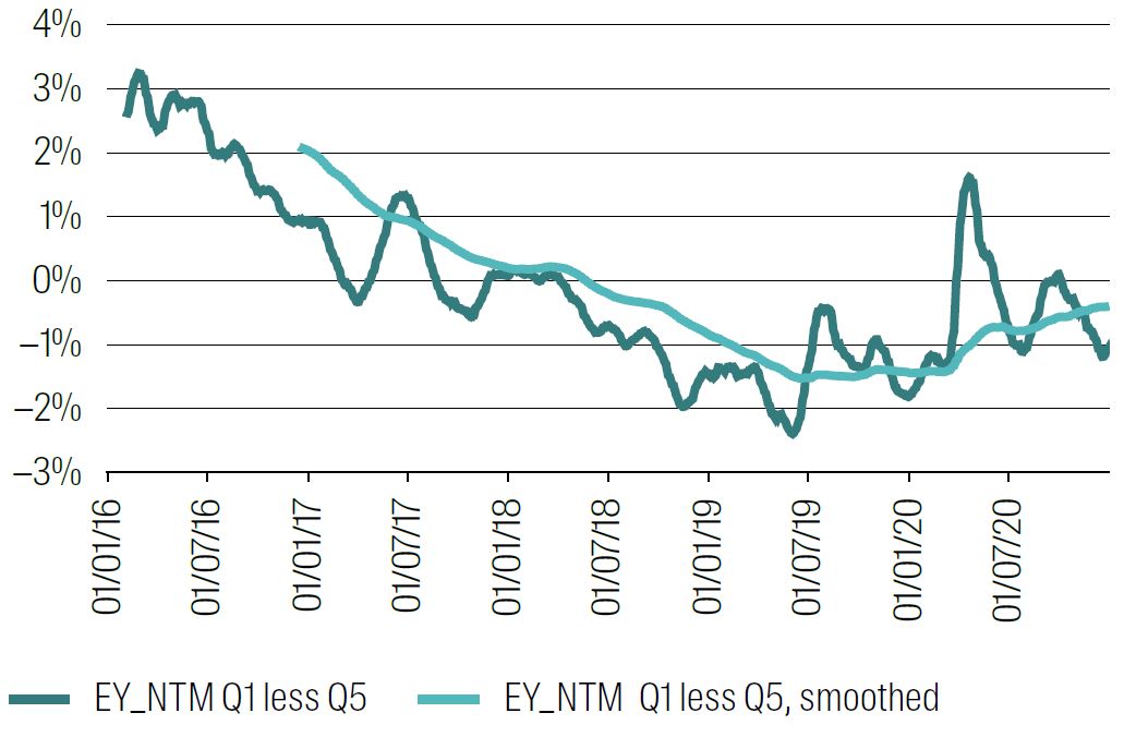
Chart 6 Panel C zooms in to the quant winter period – from the start of Jan 2016 to the end of Dec 2020.⁵ Recall that each point in the chart is the Value tilt that will maximise returns over the next 250 days.

Chart 6 Panel C: Value exposure in oracle quintile spread Q1–Q5

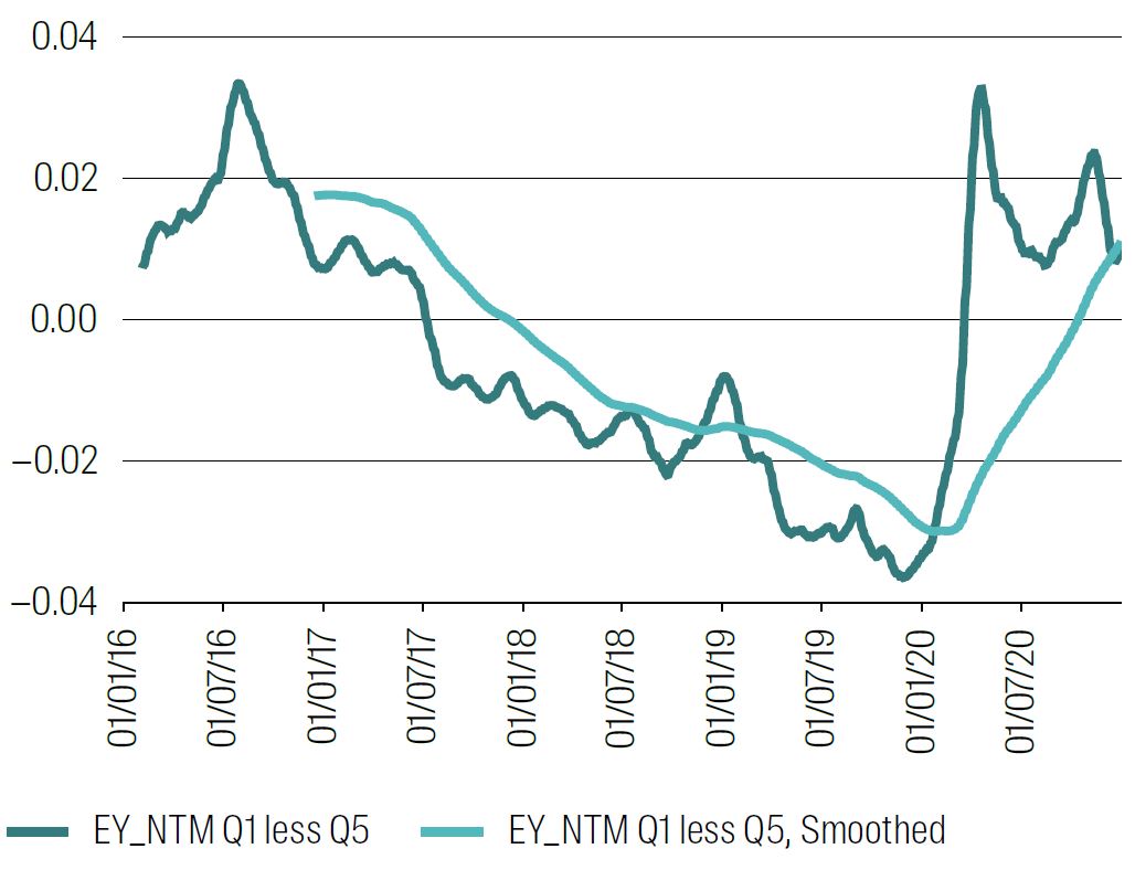
1 Jan 2016 to 1 Jan 2021.
Again, smoothing is via 25 day and 250 day rolling averages.
Source: RQI Investors, MSCI, 2025

We see the essence of the quant winter here. At the beginning of 2016 we would want to hold a positively tilted Value portfolio to get the best return over the following 250 days. But this tilt rapidly declined, went negative and remained strongly negative for the quant winter period. In other words, we would want to tilt aggressively away from Value for perhaps two years to take advantage of our oracle’s knowledge of the future, and that tilt became stronger as the period went on. This tilt only rebounded back to value during late 2020.

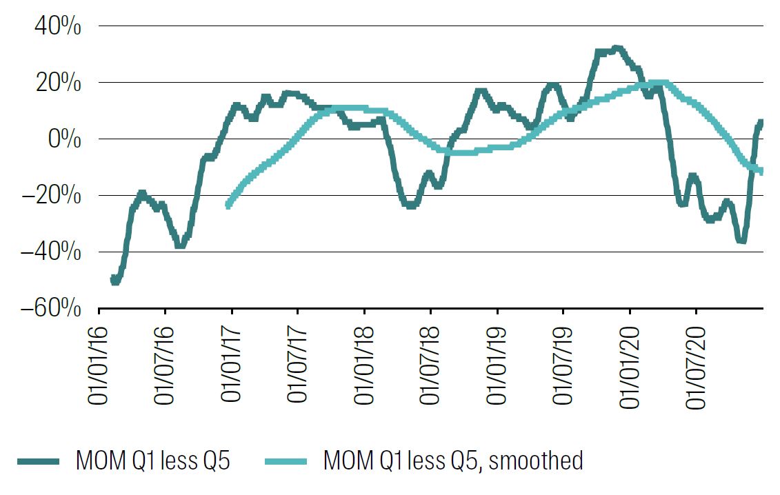
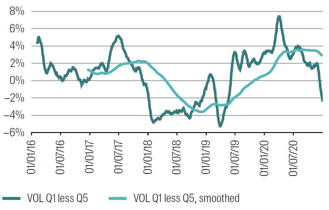
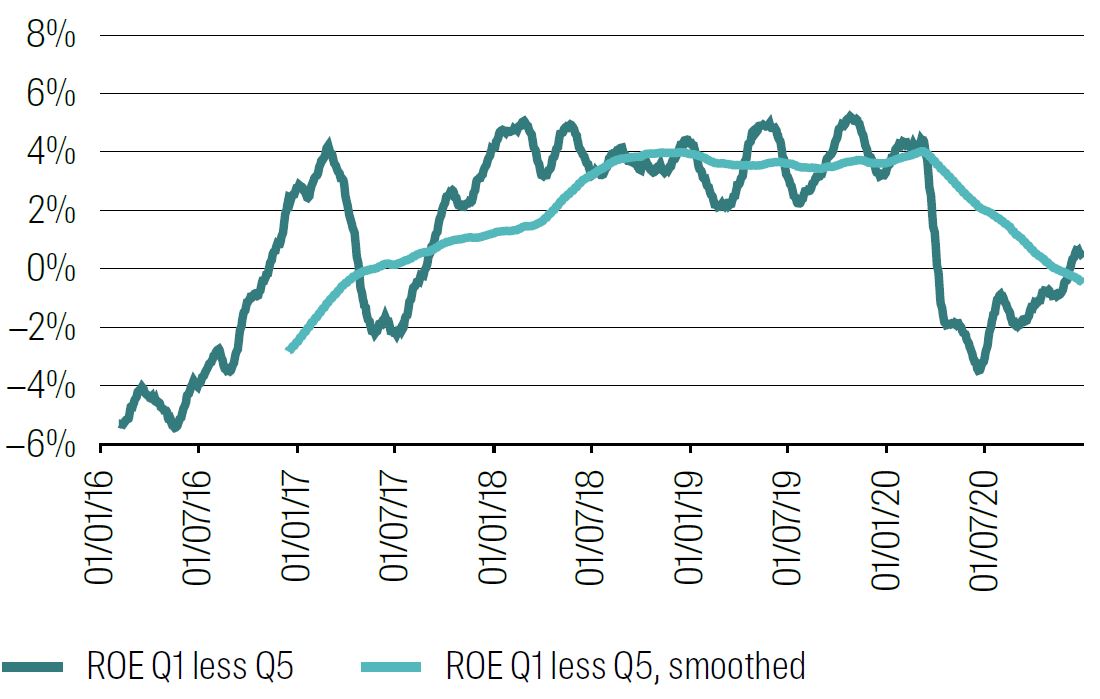
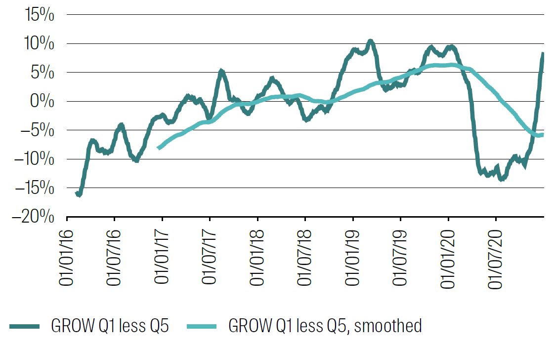
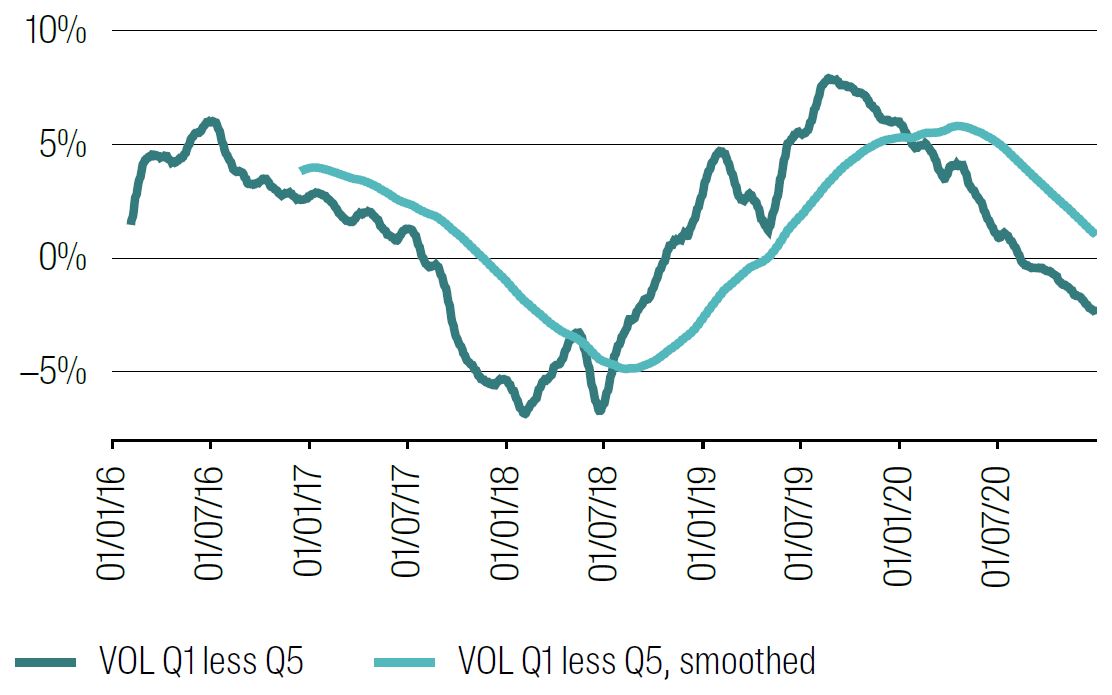
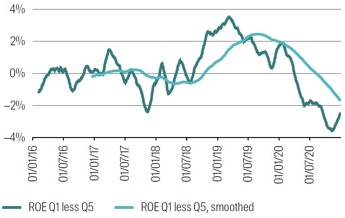
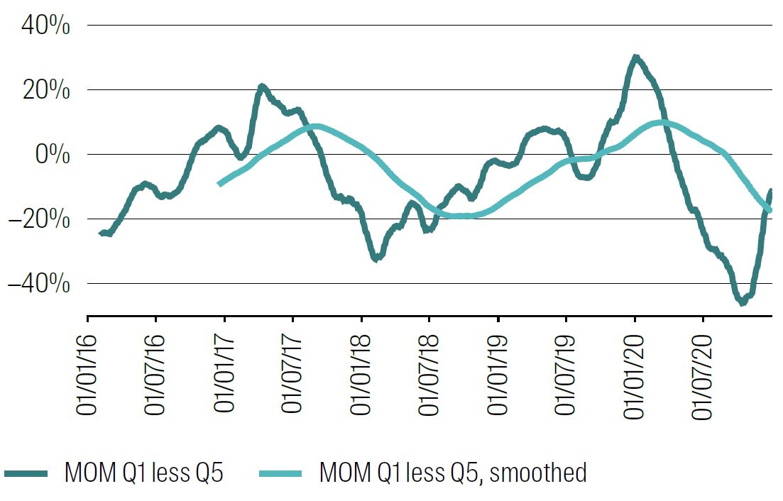
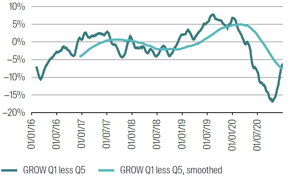
Chart 7 repeats this for the other factors – Volatility, Momentum, Quality and Growth.

Chart 7 Panel A: Volatility exposure in oracle quintile spread Q1–Q5

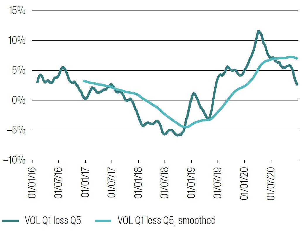
1 Jan 2016 to 1 Jan 2021.
Smoothing is via 25 day and 250 day rolling averages.
Source: RQI Investors, MSCI, 2025.

Chart 7 Panel B: Momentum exposure in oracle quintile spread Q1–Q5

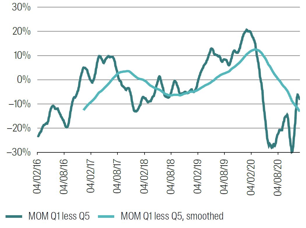
1 Jan 2016 to 1 Jan 2021.
Again, smoothing is via 25 day and 250 day rolling averages.
Source: RQI Investors, MSCI, 2025.

Chart 7 Panel C: Quality exposure in oracle quintile spread Q1–Q5

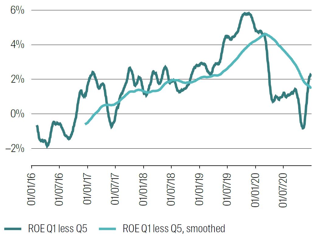
1 Jan 2016 to 1 Jan 2021.
Again, smoothing is via 25 day and 250 day rolling averages.
Source: RQI Investors, MSCI, 2025.

Chart 7 Panel D: Growth exposure in oracle quintile spread Q1–Q5

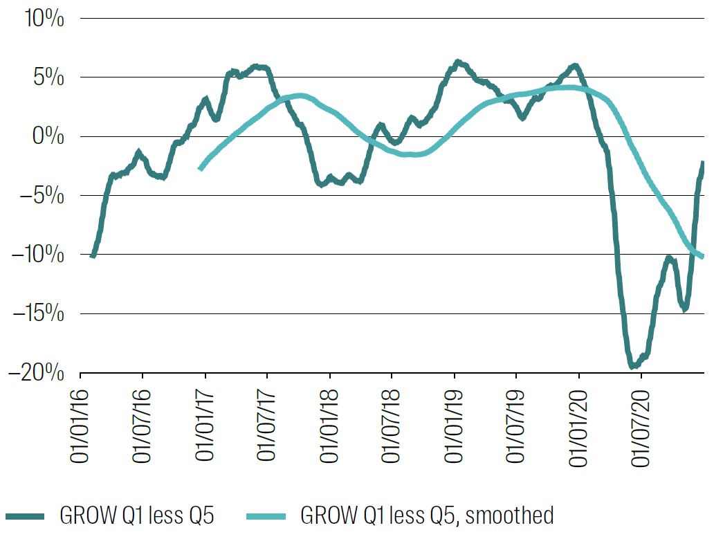
1 Jan 2016 to 1 Jan 2021.
Again, smoothing is via 25 day and 250 day rolling averages.
Source: RQI Investors, MSCI, 2025.

Knowing return quintiles 250 days ahead during the quant winter would have led us to:

• An increasingly large tilt towards expensive stocks.
• Have a mostly neutral momentum tilt.
• Start with low vol but switch to high vol later.
• Tilt towards better quality stocks.
• Have a mostly neutral growth tilt.

The first and last here are a little surprising. More usual behaviour has underperformance of Value coupled with strong momentum and/or growth. We do not see this here – it would not have helped to be overweight momentum or growth during the quant winter, despite the selloff of Value.⁶

Quality is quite clear – an overweight to ROE would almost always have been preferred, and that overweight increased over the quant winter period. Volatility is more nuanced: a tilt to low vol would have paid off in the first half of the quant winter but then good performance would have demanded a rotation to high volatility stocks – which is against the usual application of that factor.

The quant winter was not just a US effect: it was felt worldwide. Chart 8 below repeats Chart 5 Panel C for Australia and for Emerging Markets.⁷

Chart 8 Panel A: Value in the quant winter period in Australia (S&P 300 benchmark)

1 Jan 2016 to 1 Jan 2021.
Smoothing is via 25 day and 250 day rolling averages.
Source: RQI Investors, S&P, 2025.

Chart 8 Panel B: Value in the quant winter period in Emerging Markets (MSCI EM benchmark)

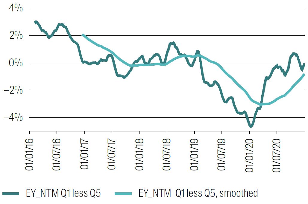
1 Jan 2016 to 1 Jan 2021.
Again, smoothing is via 25 day and 250 day rolling averages.
Source: RQI Investors, S&P, 2025.

In Australia, the quant winter effect in Value was seen in the same way as other Developed Markets, although it was not as pronounced and did not rebound in the same way. In Emerging Markets, the effect is present, just much later, deeper and for a shorter period. There is a sharp rotation away from Value at the end of 2019, which reverts quickly.

Is another quant winter likely?

As noted earlier, we don’t like the term “quant winter” very much. While it identifies the period colourfully and well, it suggests in some form that quant models are seasonal, that there might also be a quant spring, summer and autumn. This is misleading – quant models are designed to be consistent over economic cycles and have generally shown themselves to do this. The term “quant vacuum” might be better – as we know, nature abhors a vacuum.

The critical question – whatever we call this period – is the likelihood of it all happening again. That is, how likely is it that one factor will underperform sharply for an extended period, while other factors do not compensate?

We would say this is very unlikely as the circumstances which led to it were very unusual both in scale and confluence. Value significantly underperformed due to a combination of low interest rates (supporting growth) and an apparent generational step change in technology, which is highly concentrated in a few stocks. The bright new technology promised (and still promises) huge change to the economy, and the market reflected this hope with sharply increased valuation multiples (without the corresponding increase in earnings).

Quality (measured as ROE) paid off, but it was expensive. Momentum did not pay off ‑ the move may have been too concentrated. Growth did not pay off because it was not growth in earnings but a growth in multiples that was behind it. Volatility payoff was, well, volatile.⁸

In summary, the set of circumstances leading to this period was unusual and seems to have a low probability of being repeated.

Nevertheless, if such a thing were to reoccur, much the same outcomes would play out. Quant models based on these factors would almost certainly underperform again.

We would make two recommendations to help mitigate the impact of future signal vacuums like this. They seem obvious in hindsight but are critical to a high‑quality quant process.

1. Avoid overuse of generic quant factors and diversify your inputs

Quant managers stress diversification in all manner of issues, especially in portfolio construction. This should extend to diversification across signals of course, and most notably between more generic and more idiosyncratic factors. This is not to say that more generic alpha factors should be excluded – indeed, strong long‑term returns can be gained from positive tilts to well‑known momentum, value and quality factors. But balance is required with idiosyncratic ideas that are additive, differentiated and harder to crowd or arbitrage out.

2. Diversify the output factor exposures through better portfolio construction

One of the strongest lessons learned from the period of quant underperformance at the GFC was that even if alpha ideas are somewhat different, implementation of them was sufficiently similar to cause portfolios to perform in sync with each other, especially when the market was selling off. So, a lot of work has gone into understanding how to add value through better portfolio construction to transfer ideas into portfolios more efficiently. Clearly this is a way to reduce exposure to any prospective future quant factor drawdowns, although it is unlikely that we can fully immunise ourselves.

¹ In the simplest sense, valuation multiples, or using more complex models like residual income or machine learned models.

² Again, note the convention that Q1 is good and Q5 is bad.

³ This is not a ground‑breaking idea, but it does quantify the potential benefits (or losses) and shows the time varying exposure required to achieve those benefits.

⁴ We choose cap‑weighted returns rather than equally weighted as they are more representative of actual portfolios.

 ⁵ We start one year earlier than in the first paper to allow us to calculate a 250‑day future window and to see the runup to the quant winter.

⁶ This may be a result of us using equally‑weighted factor exposures within each quintile – the apparently strong momentum and growth aspects of US tech will be diluted.

⁷ Further results for Australia and Emerging Markets – for Volatility, Momentum, Quality and Growth – appear in Appendix 1.

⁸ Consider a counterfactual for a moment – the momentum factor stops working. Prices which have trended upwards on average revert downwards, and the opposite occurs for downward trends. What could cause this?
The usual argument in favour of momentum is underreaction to news. The market takes some time to process the full impact of news or expects news to be positively serially correlated (good news follows good, bad news follows bad). For this to change we would need all news to be released at the same time and for the market to incorporate it quickly.
Not only is this unlikely from a practical point of view (markets are less efficient than in the past, if anything), human behavioural biases will still lead to extrapolation.

In the first two charters, we looked at the origins of what became known as the quant winter, how it played out and what might have caused it. We also looked at how we might have been positioned (theoretically only) if we had known something of this in advance.

In this final chapter, we look at the period from the end of this quant winter to today (actually, end of April 2025), which has been a time of strong quant alpha performance, perhaps stronger than we might have expected. Is this an unusual period, or is it a snapback of the alpha drag we have seen, or something else? To try to answer these questions, we look to contemporaneous factor returns and their correlations.

We title this chapter “Recovery” rather than something like “Quant Spring” quite deliberately, as we want to avoid this interpretation that quant is somehow seasonal.

In summary, we see that this recovery period for each factor is no stronger than other periods in the past, except perhaps for the growth factor. This is almost certainly due to ongoing performance of tech. Less common is seeing Value, Momentum and Growth all performing at the same time. Unusually, Quality has been positive but lower than in the past, suggesting that the strong return to earnings growth has been at the expense of ROE.

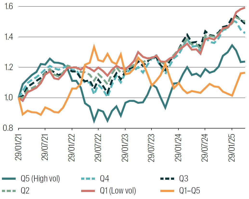
Chart 9 shows the performance of Value (as EY_NTM) from 20210101 to 20250501 – the post quant winter period.

The orange line shows the return spread between the returns of the most expensive quintile (Q5) and the best value quintile (Q1). Universe is again MSCI World ex Australia.

Chart 9: Performance of Value quintiles (measured as EY_NTM)

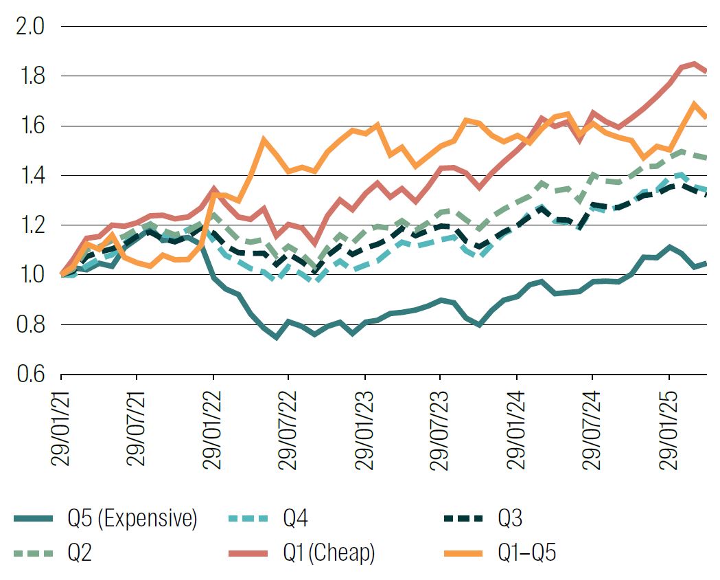
1 Jan 2021 to 1 May 2025.
Source: RQI Investors, MSCI, 2025.

Following the quant winter, in 2021, expensive stocks sold off heavily and cheap stocks rebounded strongly. From mid‑2022, expensive stocks stopped their fall and slowly recovered, at a slightly slower pace to the cheapest stocks, so the spread return growth slowed and was more volatile but did not revert for any extended period. In short, value rebounded and has continued to perform moderately well. The performance during the quant winter did not reappear.

Chart 10 shows the performance of the other quant factors we have discussed (Quality, Momentum, Growth and Volatility) over the same post‑quant‑winter period. Apart from a selloff at the end of the quant winter, and a small selldown in mid‑2022, momentum had a strong run, especially over the last two years.

Likewise, and following from the good performance during the quant winter, Quality has had continued strong performance, with no drawdowns of note and flat performance for the last 6 months or so.

After an initial slowdown, Growth has also been very strong and consistent, with high Growth stocks performing very well. Volatility has had much less direction – a strong reward to low vol as highest volatility stocks sold off heavily, and then a gradual pullback as high volatility stocks recovered.

Chart 10 Panel A: Performance of Momentum quintiles (measured as MOM12ML1M)

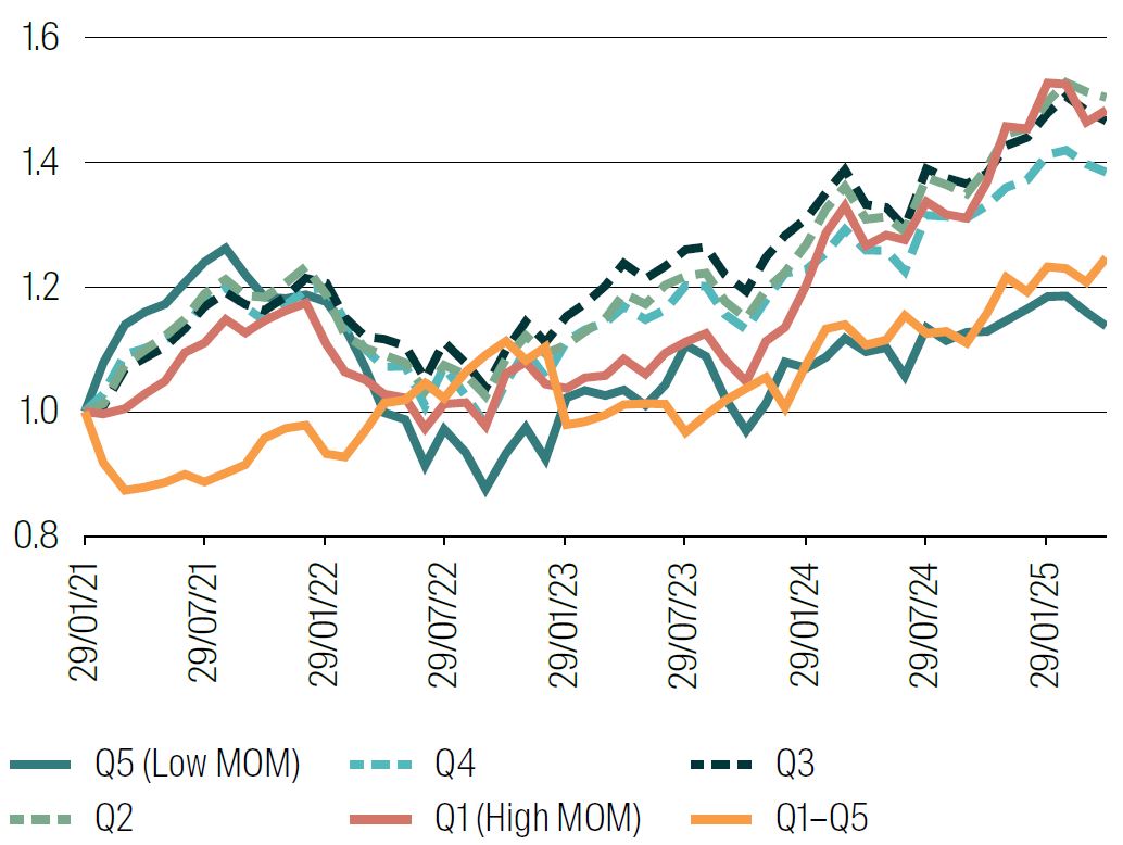
1 Jan 1 2021 to 1 May 2025.
Source: RQI Investors, MSCI, 2025.

Chart 10 Panel B: Performance of Quality quintiles (measured as ROE)

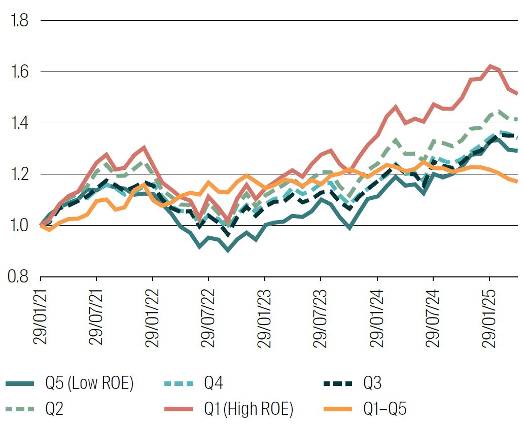
1 Jan 2021 to 1 May 2025.
Source: RQI Investors, MSCI, 2025.

Chart 10 Panel C: Performance of Growth quintiles (measured as FWD_EARNINGS_GROWTH_FY1)

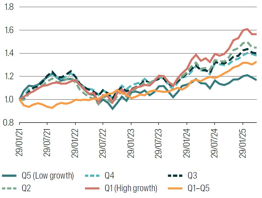
1 Jan 2021 to 1 May 2025.
Source: RQI Investors, MSCI, 2025.

Chart 10 Panel D: Performance of Volatility quintiles (measured as VOL12M)

1 Jan 2021 to 1 May 2025.
Source: RQI Investors, MSCI, 2025.

In short, we found Value, Momentum, Quality and Growth all performing positively and consistently in this period, albeit to different levels. Only a tilt to low volatility has not been rewarded the same way – it is positive but very episodic. Having these more generic quant factors perform well together is somewhat unusual, but given the preceding underperformance during the quant winter, a recovery was certainly expected.

Chart 11 below shows the correlation of three pairs of factor returns from the start of the quant winter period to today.¹

Chart 11: 24-month rolling correlation of factor Q1–Q5 return spreads

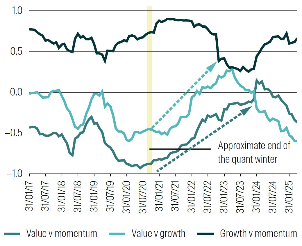
Jan 2017 to Apr 2025.
Source: RQI Investors, MSCI, 2025.

We know from experience that the Value x Momentum pair and the Value x Growth pair tend to be negatively correlated in history. Indeed, we saw something of this (and how it varied) in Table 1. What is striking about Chart 11 is the strong increase in correlation of these two pairs from the end of the quant winter until mid‑2023 and early 2024. In the case of Value x Growth, correlation trended up strongly until it was positive for the end of 2022 and the beginning of 2023. At this point, the trend reversed sharply. The same can be said for the Value x Momentum pair: while never positive the recovery is consistent until early 2024 when it too reverses.

We do not really see this is in the Growth x Momentum pair, which tells us that it is the recovery behaviour of Value that is driving it. Growth and Momentum remain strongly positive correlated throughout (with some variation).

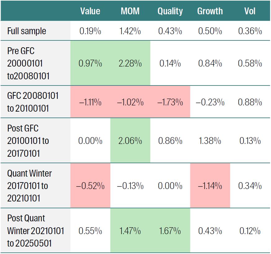
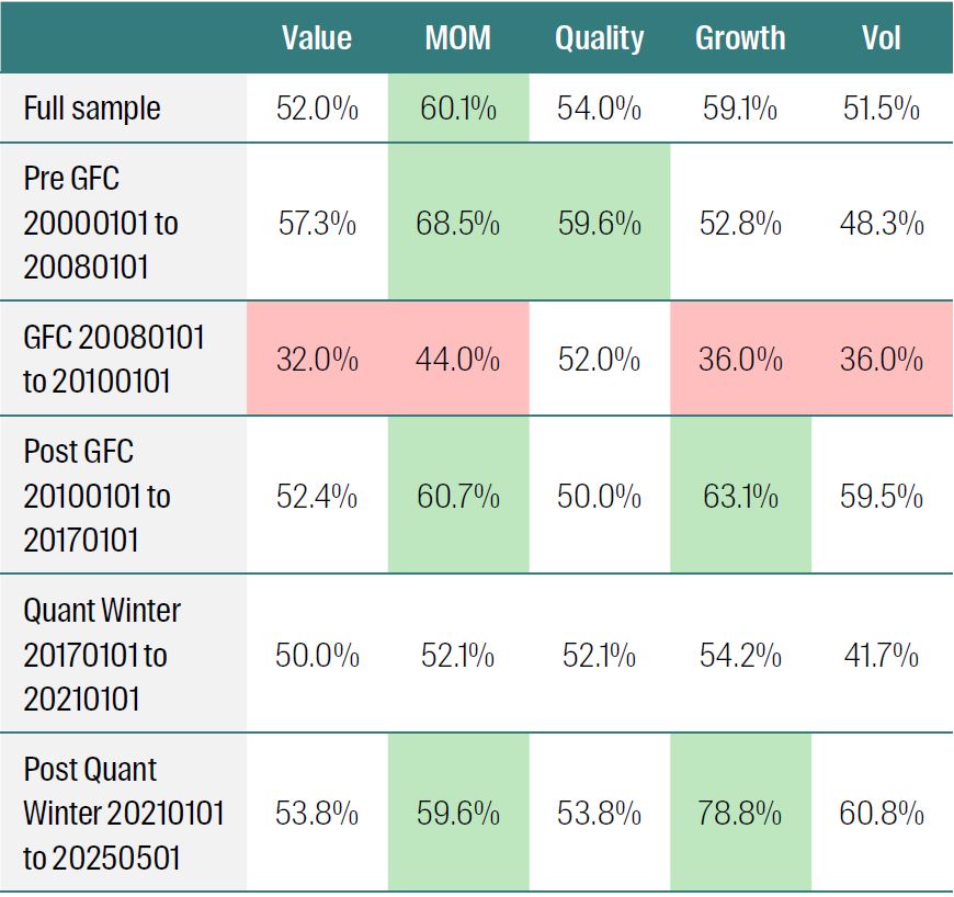
Table 2 Panel A shows that average Q1–Q5 return spread for each of five factors of interest in various samples – starting with the full data set from 20000101 to today and then breaking the data into five subperiods. Panel B repeats this with monthly hit rates (that is, percentage of positive months).²

The post quant winter period is not remarkably different in average monthly spread return to other periods or in monthly hit rate, except perhaps that Quality has been less strong and with a lower hit rate than in the past. Value rebound has been large, but on a par with the pre GFC period. Growth has been strong and consistent recently. Volatility return and hit rate appear good, but this masks the episodic nature of these returns, as we saw in Chart 10 Panel D. Outside of the GFC, Momentum has been strong.

Table 2 Panel A: Average monthly Q1–Q5 return spreads for each factor at different periods.

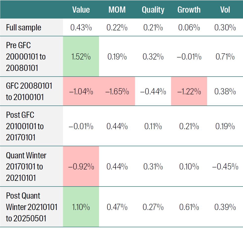
Source: RQI Investors, MSCI, 2025

Table 2 Panel B: Monthly hit rates for each factor at different periods

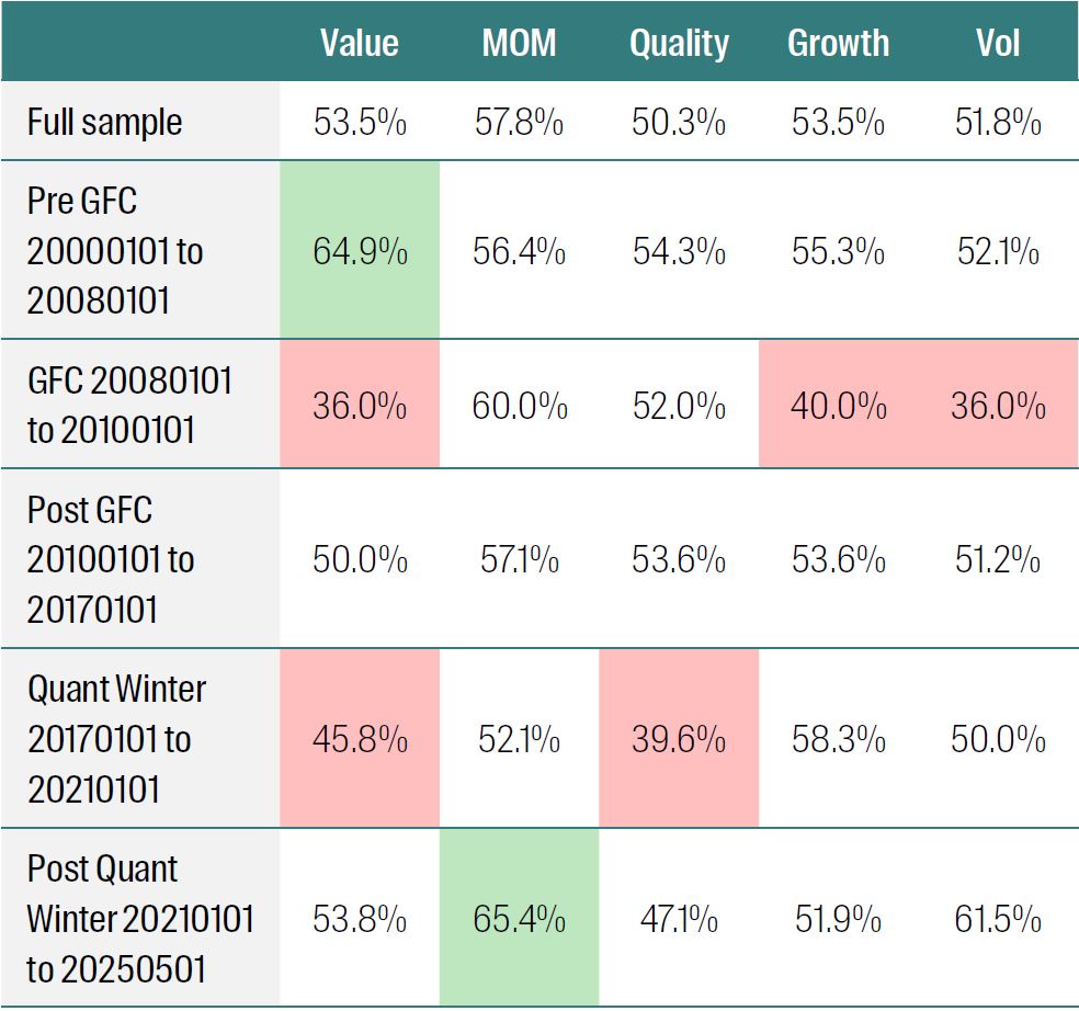
Source: RQI Investors, MSCI, 2025

¹ Correlations are 24‑month rolling and are of the return spreads between highest (Q5) and lowest (Q1) factor scores.

² Australian and Emerging Market Tables appear in the Appendix for completeness.

Here we chart the factor exposures for the Q1‑Q5 spread in oracle return forecasts, for Australia and Emerging Markets. The period is just the quant winter, as above.

Recall that these charts show the optimal factor tilt required to capture the Q1‑Q5 spread as indicated by our oracle. By taking this tilt the factor will extract the spread between the best performing quintile (Q1) and the worst (Q5) over the next 12 months.

For the ASX300

As noted above, the quant winter also arrived in Australia, but it was not as severe as for other developed markets – nor did it revert so strongly. That is, the optimal tilt to factors (to capture the maximum return) was as follows:

• Neutral to slight positive momentum.
• Start with low vol but switch to high vol later.
• Consistent tilt towards better quality stocks.
• Neutral to slight positive growth.

Charts A1: Factors in the quant winter period in Australia (ASX300 benchmark) – Momentum Exposure

Source: RQI Investors, S&P, 2025.

Charts A1: Factors in the quant winter period in Australia (ASX300 benchmark) – Volatility Exposure

Source: RQI Investors, S&P, 2025.

Charts A1: Factors in the quant winter period in Australia (ASX300 benchmark) – Quality Exposure

Source: RQI Investors, S&P, 2025.

Charts A1: Factors in the quant winter period in Australia (ASX300 benchmark) – Growth Exposure

Source: RQI Investors, S&P, 2025.

For Emerging Markets

As for the Value exposure, Emerging Markets did not see the quant winter in the same way as developed markets. A neutral tilt to value gained the greatest returns in 12 months, only requiring a sharp expensive positioning in late 2019 for a short time.

The Volatility tilts were quite pronounced – low vol first the high vol was required to capture the best return in 12 months. Quality and growth were quite neutral, while Momentum exposure swung sharply from long to short and back to long. Again, unlike developed markets, there is a large swing away from Quality, Growth and Momentum as the quant winter period ends.

Chart A2: Factors in the quant winter period in Emerging Markets (MSCI EM benchmark) – Volatility Exposure

Source: RQI Investors, S&P, 2025.

Chart A2: Factors in the quant winter period in Emerging Markets (MSCI EM benchmark) – Quality Exposure

Source: RQI Investors, S&P, 2025.

Chart A2: Factors in the quant winter period in Emerging Markets (MSCI EM benchmark) – Momentum Exposure

Source: RQI Investors, S&P, 2025.

Chart A2: Factors in the quant winter period in Emerging Markets (MSCI EM benchmark) – Growth Exposure

Source: RQI Investors, S&P, 2025.

Australian and Emerging Market results for the post quant winter period.

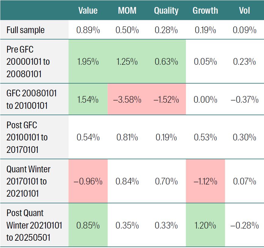
Table A1 Panel A: Average monthly Q1–Q5 return spreads for each factor at different periods (Australia)

Source: RQI Investors, S&P, 2025

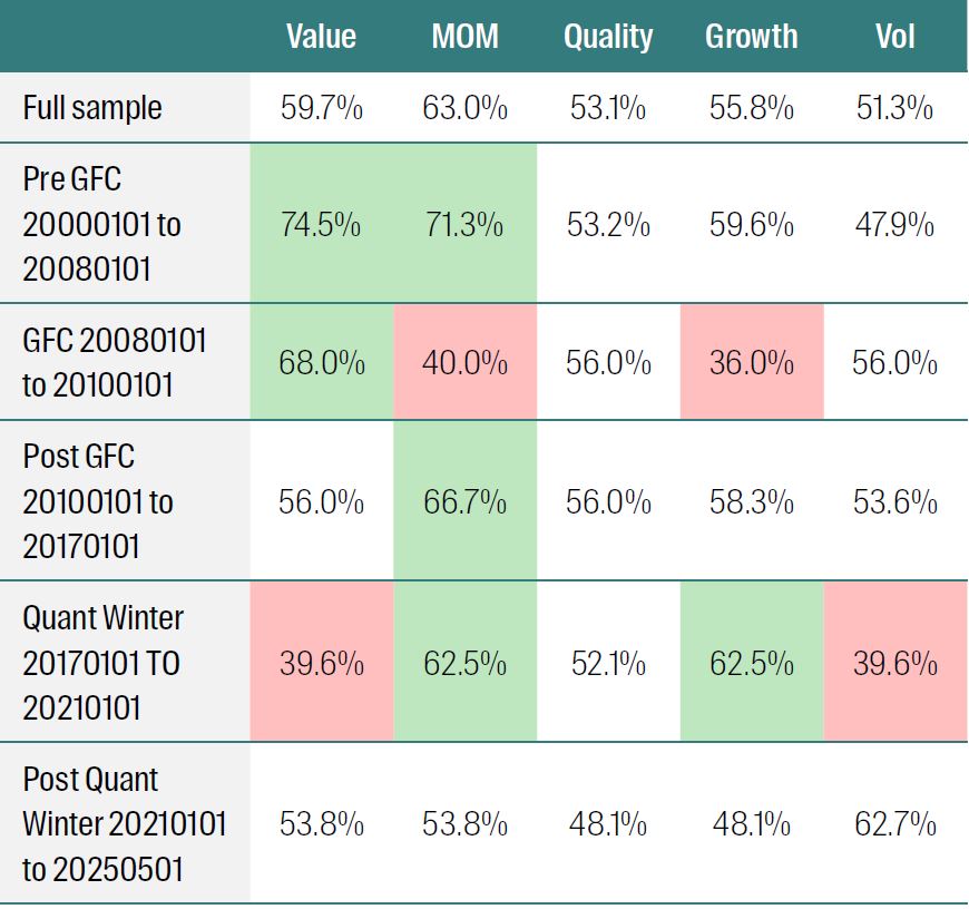
Table A1 Panel B: Monthly hit rates for each factor at different periods (Australia)

Source: RQI Investors, S&P, 2025

Table A2 Panel A: Average monthly Q1–Q5 return spreads for each factor at different periods (Emerging Markets)

Source: RQI Investors, MSCI, 2025

Table A2 Panel B: Monthly hit rates for each factor at different periods (Emerging Markets)

Source: RQI Investors, MSCI, 2025

RQI Investors Real Insights: Lessons from the Quant Winter

In this episode we explore RQI Investors latest research “Lessons from the Quant Winter”,  a comprehensive report that examines the challenging period from 2018 to 2020 when quant strategies faced significant headwinds. We unpack the causes behind this underperformance, the impact on markets (especially in Australia and other developed economies), and the surprising rebound post-COVID. We explore the intersection of human expertise and advanced technology, brought to life through an AI-generated voice.