What is Prospect Theory?
Imagine you are offered two $50 notes, but if you take both you must immediately destroy one of them (e.g. burn it) or give it away. Or you can just take one $50 note. Which would you choose?
Your wealth – in a purely rational and objective world – will increase by exactly the same amount, so you would be indifferent. However, you may express a preference for one of the options above the other. What does that tell you?
Most people, it seems, will choose the second option. The pain of wasting $50 matters in the decision, even though it actually makes no difference in wealth. While this seems irrational, it reflects many decisions and behaviour that we observe in everyday life. Behaviour like this is at the centre of the idea of Prospect Theory, which was developed by Kahneman and Tversky (1979 and 1992)1,2.
In their studies, Kahneman and Tversky gathered a group of university students and academics and gave them two situations to consider. The situations separately considered the attitude individuals have towards gains and losses.
In the first situation (gains), each person was notionally given $1000, and could choose one of two options:
A 50% chance of gaining $1000, 50% chance of gaining $0
B 100% chance of gaining $500
Note that the expected gain is $500 in both cases. A huge majority of the sample chose B.
In the second situation (losses), each person was notionally given $2000, and could choose one of two options:
C 50% chance of losing $1000, 50% chance of losing $0
D 100% chance of losing $500
Note that the expected loss is $500 in both cases. However, now a majority of the sample chose C.
In other words, individuals prefer certainty in gains even if there is a chance of higher returns but are prepared to take a chance to mitigate losses, even if they might potentially be worse off. That is, the concern of a loss is greater (per dollar) than the equivalent elation of a gain. In an investment sense: investors are more loss-averse than they are gain-seeking.
One last point here – the choice of the name “prospect theory” is a little unclear. It was named like this (by Kahneman and Tversky) because it tries to capture how people evaluate the various options or “prospects” that they encounter. In an environment when various choices are available, and the outcomes are uncertain, the payoffs and their likelihoods can be thought of as the “prospects” of that environment.
Conventional economic theory assumes individuals are perfectly rational in their decision making under uncertainty. This is usually known as expected utility theory. It is different to prospect theory, which represents more how people actually behave (“irrationally”?) rather than how they are expected to behave. For example, prospect theory considers options relative to a reference point – see below – rather than in terms of absolute wealth.
Examples in real life
This is contrary to the long-accepted theory that losses and gains are felt equally. While controversial, it has been shown to appear in many human pursuits. Here are some examples:
Insurance: As we will see later, prospect theory implies that we tend to overweight low probability events, like a house fire or some other catastrophe. We are willing to pay insurance premiums for these highly unlikely events, effectively switching a low probability large loss for a certain smaller loss. At the same time, we are less likely to purchase insurance for higher probability lower loss events, like loss or damage to a mobile phone.3
In summary, as predicted by prospect theory, we overweight low probability events, underweight high probability events and are more averse to loss than gain, and our insurance purchases follow this.
Gambling: Why are gamblers willing to bet on zero or negative expected value games in casinos?4 Think of the example of a gambler who loses $500 compared to a gambler who has won $200. The losing gambler is more likely to take on another $500 gamble (“to make up the loss”) than the winning gambler. Losses matter more than gains.
Or think of another example. Expected payoffs here are the same but because they overweight the tail probabilities, gamblers will prefer:
(A gain of $5000 with probability 0.001) over (A certain payment of $5).
(A certain loss of $5) over (A loss of -$5000 with probability 0.001).
Health: Prospect theory seems to apply to non-monetary rewards as well as monetary. It seems obvious but individuals who are less satisfied with their body shape and wish to lose weight tend to have higher risk seeking behaviour when it comes to weight loss or gain. That is, they equate weight loss (gain) with “psychological” gain (loss), and their aversion to weight gain is roughly twice their desire for weight loss (in the sample from the paper).5
Leisure and tourism: When you choose a restaurant - or a meal at a restaurant – or choose a holiday destination, do you go with what is familiar or do you “take a chance”? In the same way as for health, behavioural models like prospect theory can help to explain why people might choose one type of leisure activity (for example, how likely are people to avoid loss by choosing a “safe” venue rather than risking an unfamiliar one, and how might you identify each group?).6
Markets: In investments, a similar behaviour has been observed, which has been named the disposition effect. This is when investors sell winners too early and hold on to losers too long. We will explore this a little more below.
Editing and evaluation
Prospect theory is usually split into two stages: editing and evaluation. Other applications in different fields might use different terms - for example, editing can also be called “representation”.
The ideas are as follows:
Editing (or Representation) is where the set of possible options is considered – when we mentally collate, organise and label the data we will use to make the decision. We will also choose a reference point (e.g., current state, or some average entry price) to which we will compare likely future outcomes. This is also the stage where we assign likely probabilities to those outcomes.
There are behavioural biases inherent in this phase where we might omit data that does not seem likely or does not agree with our ideas. We might also overweight the probability of extreme events. In effect, we represent our understanding of the payoff as a set of outcomes and their probabilities as we understand them.
Evaluation (or just Valuation) is the stage where we look at the data we have gathered and decide how we might interpret or value it. We might, at this stage, decide that we are more concerned about losses than gains, and where we aim to calculate the payoffs or losses, we might achieve following a choice.
What does prospect theory look like?
Prospect theory was born from the empirical work of Kahneman and Tversky (that is, measurement, not theory). They observed behaviour that did not fit the theory and built mathematical models which better represented what they were seeing.
There were two parts to this:
The utility function of gains and losses to wealth
The overweighting of low probability events and the underweighting of higher probability events
The mathematical models they developed were as follows (from Barberis et al (2016), from now on BMW167):
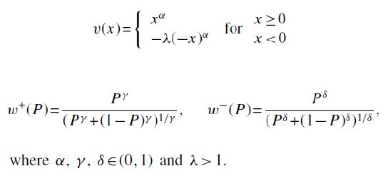
The first equation is the shape of valuation or utility function v(x) and the pair of second equations are the probability weightings w+(P) for gains and w-(P) for losses. Note that these models involve three parameters:
loss aversion (LA) via λ,
Higher λ means the curve is steeper on the loss side.
probability weighting (PW) via {γ,δ},
Higher values of γ and δ mean greater weightings to the tail probabilities.
convex/concave (CC) via α
Higher value of α increases the curvature of the utility function v(x).
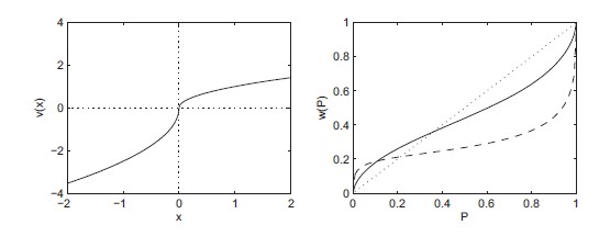
These are easier to understand in charts. Figure 1 below also comes from BMW16.
Figure 1: Prospect Theory Value and Probability Weighting functions
Source: BMW168
In the chart on the left-hand side of Figure 1, we can see that for positive values of x the value or utility achieved from increasing x reduces as x gets bigger. If x is small and increases, the increase in utility is greater than if x starts at a higher value. To understand this, think of receiving $200 and then getting another $100. The impact is meaningful. However, if you receive $1000, and then an extra $100, it has less importance.
On the other side, the story is similar but reversed. If you lose $200 and lose another $100, it is a larger effect than losing $1000 and then losing another $100.
Said another way, the impact of the loss or gain of $100 to you changes based on how much you have lost or gained already.
Finally, note that the slope of the curve for losses is greater than the slope for gains. People are more “loss averse” than they are “return seeking”. A $200 loss has greater impact (per dollar) than a $200 gain.
The probability function (right hand side of Figure 1) is next. If all outcomes (regardless of probability) are equally likely (in reality) then the true weight we should assign follows the dotted line (where δ=1). However, if you subjectively think tail probabilities (i.e., very low likelihood events) are more likely, then the curved (dashed or solid) lines are above the straight (dotted) line for low values of P, and below it for high values of P. Low probability events are overestimated for δ = 0.4 (dashed) and δ = 0.65 (solid) and high probability events are underestimated.
Note that the origin on the left-hand side chart (that is, where v and x are both zero) is the starting point for any comparison. There is no reason to think that this is an absolute position, in fact it will be different for each person. In that sense the origin is what is known as the Reference Point – all decisions are made with respect to this point. This depends entirely on the individual making the decision. The Reference Point could simply the last traded price, the entry price for a recent purchase for a single trade or even the effective price for a holding against which tax calculations are made (e.g., LIFO).
In combination, these formulas capture the essence of prospect theory. Note that this is not an economic theory, but the shapes and parameters are chosen to match what are seen in reality.
What is the disposition effect?
All of this is fine in an abstract sense but to crystallise it in the context of financial markets, we need to introduce the disposition effect. It was first identified and named by Shefrin and Statman (1985)9, 10, where it was found while looking at trading patterns of individual retail investors. The name comes from the idea that:
Investors are “predisposed” to sell winners too early and to sell losers too late, and they find evidence that this exists – and it is not a tax effect.
An example: you own stock A which has risen in value. You believe that there is still upside in the stock but timing the top is difficult, and “you never go broke taking a profit”. That is, you are aware that the price might go higher, but you are comfortable missing out and would repeat the action.
Or you own stock B which has fallen in value. You think the stock could fall further, and it could also rise again, but you decide to “hang on for the ride”. You don’t sell out because you have already absorbed the loss, and you are ok if it goes lower and would repeat the action.
Let’s place this in the theory we described above. The figures below come from Frazzini (2006)11 with some additions to clarify the ideas.
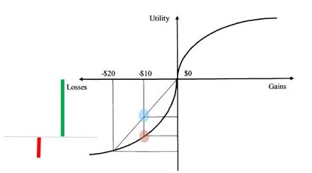
Case 1: Stock falls $10 and we don’t sell.
In the first chart below (Figure 2), we own a stock with the Reference Point at the centre or origin. The stock then falls $10 and we want to assess whether we would sell now. For simplicity, assume the next move is equally likely to be +$10 or -$10.
If risk neutral – blue dot – so we are indifferent to buying or selling.
However, if we use the Prospect Theory utility function - red dot - then the story is different.
If the stock recovers and we have not sold, the positive change in utility from continuing to hold the stock is the green bar. That is, there is significant upside to our utility if we don’t sell and the price recovers. If the stock continues to fall and we have not sold, we lose another $10 but the reduction in utility (the red bar) is smaller than the green bar.
In other words, the $10 upside means more to us than the $10 downside. If the stock is equally likely to go up or down by $10, and we do not sell, then the expected change in utility (green bar less red bar) is positive. So we don’t sell.
Figure 2: The Disposition Effect with a loss – do not sell
Source: Frazzini (2006)12
Case 2: Stock rises $10 and we sell.
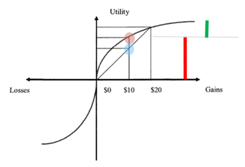
In the second chart below (Figure 3), we own a stock with the Reference Point again at the origin. The stock then rises $10 and we want to assess whether we would sell now. For simplicity, again assume the next move is equally likely to be +$10 or -$10.
If risk neutral – blue dot – so we are indifferent to buying or selling.
However, if we use the Prospect Theory utility function - red dot - then the story is different.
If the stock falls and we have not sold, the negative change in utility from continuing to hold the stock is the red bar. That is, there is downside upside to our utility if we don’t sell and the price falls.
If the stock continues to rise and we have not sold, we gain another $10 but the increase in utility (the green bar) is smaller than the red bar.
In other words, the $10 upside means less to us than the $10 downside. If the stock is equally likely to go up or down by $10, and we do not sell, then the expected change in utility (green bar less red bar) is negative. So we sell.
To summarise, even if the probability of the next price change is equally likely to be up and down, we will choose to sell if the price has already risen but not sell if it has fallen. So Prospect Theory appears to describe the disposition effect as it has been observed.
Figure 3: The Disposition Effect with a gain – sell
Source: Frazzini (2006)13
Can we trade on this? Operationalising Prospect Theory
Behavioural biases push prices away from fundamentals – e.g., selling early or late in the case of the disposition effect. Here, if prices have fallen below the individual’s reference price, the individual is less likely to sell, creating an imbalance of buying over selling so future returns will be higher. On the other hand, if prices have risen above the reference price, selling has an increased likelihood, so the resulting imbalance selling over buying means future returns will be lower.
In other words, the disposition effect appears to induce mispricing which might be able to be exploited as a source of alpha. To implement or test this, we use the Tversky-Kahneman (TK) empirical utility function v(x) which appears earlier, on page 4. Using it we can write a resulting valuation function based on the behavioural biases and its parameters (see BMW16). The components of the valuation function are (as we have noted earlier) two parts – representation and valuation.
BMW16 write this down using equations directly from TK, and give a simple example, which can potentially be expanded and exploited. They write down a valuation function as a weighted average of the values of possible outcomes:
The values come from the TK utility function v(x)
The possible outcomes are the possible set of x values, weighted by the TK probability function.
The valuation function is therefore written as:

where p = probabilities of each possible outcome
w+ = weights for outcomes if positive
w- = weights for outcomes if negative
The TK theory then says:
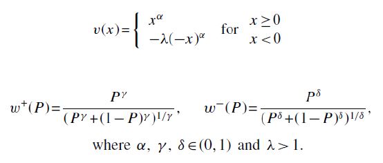
Recall: These models involve three things – loss aversion (LA) via λ, probability weighting (PW) via {γ,δ} and convex/concave (CC) via α. Authors use α = 0.88, λ = 2.25, γ = 0.61 and δ = 0.69.
Now, what is the set of possible outcomes x and their probabilities p? That is, what is the representation that an investor might form?
In some ways this is most important part of the process, as each investor may have a different set of data and probability weightings they choose. BMW16 choose a simple example to illustrate their point, and the results they achieve suggest that this might be meaningful. They choose to represent each stock as an equally weighted last 60 months of returns, that is:

You or I might find this overly simplistic and might suggest using (a) a short window, (b) decaying importance over time or (c) highlighting specific events. However, the authors show that despite its simplicity, this simple representation has some power.
The Valuation model becomes:
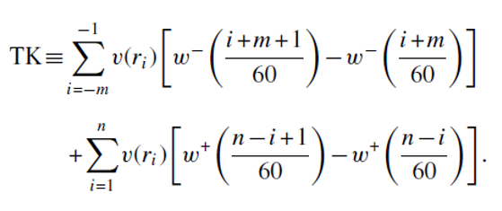
The idea is that a stock with a higher value of TK is more likely to be purchased, which overvalues the stock so that future returns will be lower. Conversely, lower values of TK suggest that investors are more likely to sell, which undervalues the stock so that future returns will be higher.
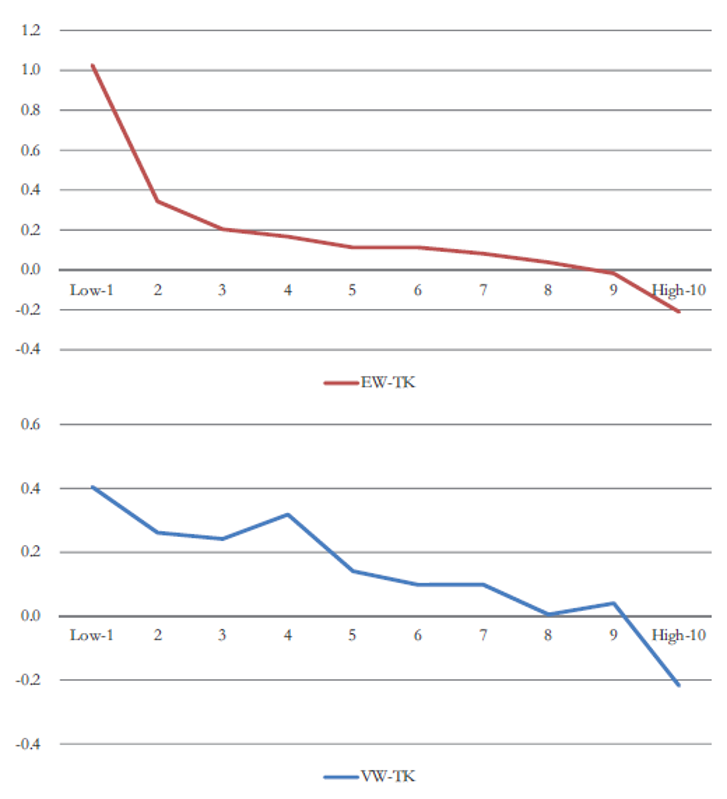
This is exactly what they find – see Figure 4 below, which comes from the Barberis et al (2016) paper. It is the excess return14 generated from each decile of TK in their sample. The top chart is equally weighted return in each decile, and the bottom chart is the same returns but now weighted by market cap. Low values of TK do indeed show excess positive returns, while higher values of TK do indeed show excess negative returns.
There is a more or less monotonic reduction in returns as TK value increases, which further supports the results. The return spread between bottom and top decile is high, so a portfolio that is long the lowest decile of TK values and short the highest decile will earn significant monthly returns.
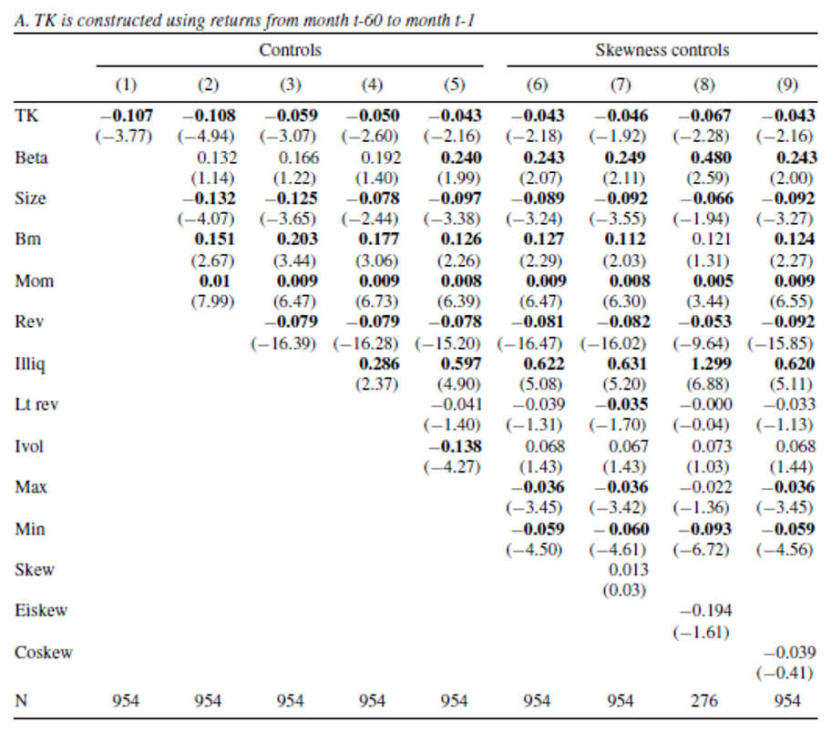
Table 1 below is from Barberis et al (2016). It shows that if we test these long-short returns against a variety of other common factors as controls (beta, size, idiosyncratic volatility, illiquidity and so on)15 that the excess returns remain strong. Model (9) - which has the broadest set of controls – still shows a negative and statistically significant return to TK. (Negative coefficient is expected, as higher TK values are expected earn lower returns.)
Figure 4: Alpha in TK deciles (equally weighted EW and market cap or value weighted VW)
Source: BMW1616
Table 1: Fama-MacBeth cross sectional regressions of stock returns on a variety of factors, including TK. The aim is to see if each new factor added detracts from relationship between TK and returns.17
Source: BMW1618
One open question here comes from the following observations:
stocks which have fallen will have lower motivation for holders to sell, which means that prices might rise.
stocks which have risen will have higher motivation for holders to sell, which means that prices might fall.
So, implementation of this idea might be captured by a strategy which buys stocks which have fallen and sells stocks which have risen. In other words, it may look like a price reversal/value or anti-momentum strategy. The extent to which this alpha idea might be captured by one of these existing alpha signals is an open question. The results on Table 1 suggest that it may be additive – but this remains to be seen in practice.
Summary and Conclusions
Humans have behavioural tendency to be risk averse to gains and risk seeking for losses. In markets terms we might call this “taking profits” and “riding losses”. Kahneman and Tversky, in a number of research papers, developed an empirical model which captures this behaviour, and named the effect Prospect Theory. Individuals (they say) mentally build a representation of the likely set of outcomes (“editing”) and then weigh up the valuation of each outcome (“evaluation”).
In this, they note four things:
Individuals have a reference price with which they measure price moves.
They are more sensitive to losses than gains.
They tend to upweight the likelihood of extreme events.
Gains (losses) have concave (convex) utility.
In finance, this potentially manifests itself in what is known as the disposition effect, where holders of stock crystallise gains too early and realise losses too late.
Prospect theory and the disposition effect then lead to a direct application for potential alpha generation, as has been discussed above via the paper by Barberis et al (2016). Results suggest that there might be an opportunity to generate alpha by taking advantage of this mispricing:
Tilting towards stocks which have a low prospect theory value (meaning that sellers have potentially withdrawn) as they are likely to have higher returns.
Tilting away from stocks which have a high prospect theory value (meaning that selling has been accelerated) as they are likely to have lower returns.
We can see that this idea has some close positive correspondence with price reversal strategies like value and against models like momentum. However, empirically tested alpha seems strong and resilient to the impact of other common factors.
1 Kahneman and Tversky (1979), Econometrica, “Prospect Theory: An Analysis of Decision under Risk”.
Tversky and Kahneman (1992), Journal of Risk and Uncertainty, “Advances in Prospect Theory: Cumulative Representation of Uncertainty”
2 Note that this is not the same proposal as that discussed in Thinking Fast and Slow, another work by these authors. That work describes how we balance decisions between “first impressions” (fast) and “after further consideration” (slow), clearly not the same idea as Prospect Theory.
3 https://thedecisionlab.com/biases/loss-aversion
4 Barberis (2011) NBER working paper, “A Model of Casino Gambling”.
5 For example, Lim and Bruce (2015), Frontiers in Psychology: “Prospect theory and body mass: characterising psychological parameters for weight related risk attitudes and weight-gain aversion”
6 See for example Lin et al (2024) University of Essex working paper, “An Assessment of Prospect Theory in Tourism Decision-Making Research.”
7 Barberis, Mukherjee and Wang (2016), Review of Financial Studies, “Prospect Theory and Stock Returns: An Empirical Test”
8 Barberis, Mukherjee and Wang (2016), Review of Financial Studies, “Prospect Theory and Stock Returns: An Empirical Test”
9 Shefrin and Statman (1985), Journal of Finance, “The Disposition to Sell Winners Too Early and Ride Losers Too Long: Theory and Evidence”
10 There are many other examples in the literature which demonstrate the disposition effect. An early sample:
Heisler (1994), Review of Futures Markets, “Loss aversion in a futures market: An empirical test”
Weber and Camerer (1998), Journal of Economic Behaviour and Organisation, “The disposition effect in securities trading: An experimental analysis”
Odean (1998), Journal of Finance, “Are investors reluctant to realize their losses?”
Odean (1999), American Economic Review, “Do investors trade too much?”
Heath, Huddart and Lang (1999), Quarterly Journal of Economics, “Psychological Factors and Stock Option Exercise”
11 Frazzini (2006), Journal of Finance, “The Disposition Effect and Underreaction to News”
12 Frazzini (2006), Journal of Finance, “The Disposition Effect and Underreaction to News”
13 Frazzini (2006), Journal of Finance, “The Disposition Effect and Underreaction to News”
14 Excess to the Fama-French-Carhart four factor model (Carhart (1997), Journal of Finance, “On Persistence in Mutual Fund Performance”). All US stocks from 1926 to 2010.
15 These are known widely in quantitative finance research as Fama-MacBeth regressions after the original paper that suggested their use. (Fama and MacBeth (1973). Journal of Political Economy, "Risk, Return, and Equilibrium: Empirical Tests".)
16 Barberis, Mukherjee and Wang (2016), Review of Financial Studies, “Prospect Theory and Stock Returns: An Empirical Test”
17 Beta is five-year monthly beta. Size is log(market cap). BM is log(book to market). Mom is 12-month price momentum (less most recent month). Rev is most recent month’s return. Illiq is Amihud’s illiquidity measure, which is absolute price change divided by volume, LT Rev is last 60 months’ return, Ivol is idiosyncratic return volatility, Max and Min are the largest and smallest daily returns in the last month, and the skew metrics measure the skewness of return distributions of stocks
18 Barberis, Mukherjee and Wang (2016), Review of Financial Studies, “Prospect Theory and Stock Returns: An Empirical Test”
Read our latest insights
Important Information
This material is for general information purposes only. It does not constitute investment or financial advice and does not take into account any specific investment objectives, financial situation or needs. This is not an offer to provide asset management services, is not a recommendation or an offer or solicitation to buy, hold or sell any security or to execute any agreement for portfolio management or investment advisory services and this material has not been prepared in connection with any such offer. Before making any investment decision you should consider, with the assistance of a financial advisor, your individual investment needs, objectives and financial situation.
We have taken reasonable care to ensure that this material is accurate, current, and complete and fit for its intended purpose and audience as at the date of publication. No assurance is given or liability accepted regarding the accuracy, validity or completeness of this material and we do not undertake to update it in future if circumstances change.
To the extent this material contains any expression of opinion or forward-looking statements, such opinions and statements are based on assumptions, matters and sources believed to be true and reliable at the time of publication only. This material reflects the views of the individual writers only. Those views may change, may not prove to be valid and may not reflect the views of everyone at First Sentier Investors.
About First Sentier Investors
References to ‘we’, ‘us’ or ‘our’ are references to First Sentier Investors, a global asset management business which is ultimately owned by Mitsubishi UFJ Financial Group. Certain of our investment teams operate under the trading names AlbaCore Capital Group, FSSA Investment Managers, Stewart Investors, RQI Investors and Igneo Infrastructure Partners, all of which are part of the First Sentier Investors group.
We communicate and conduct business through different legal entities in different locations. This material is communicated in:
- Australia and New Zealand by First Sentier Investors (Australia) IM Ltd, authorised and regulated in Australia by the Australian Securities and Investments Commission (AFSL 289017; ABN 89 114 194311)
- European Economic Area by First Sentier Investors (Ireland) Limited, authorised and regulated in Ireland by the Central Bank of Ireland (CBI reg no. C182306; reg office 70 Sir John Rogerson’s Quay, Dublin 2, Ireland; reg company no. 629188)
- Hong Kong by First Sentier Investors (Hong Kong) Limited and has not been reviewed by the Securities & Futures Commission in Hong Kong. First Sentier Investors, FSSA Investment Managers, Stewart Investors, RQI Investors and Igneo Infrastructure Partners are the business names of First Sentier Investors (Hong Kong) Limited.
- Singapore by First Sentier Investors (Singapore) (reg company no. 196900420D) and this advertisement or material has not been reviewed by the Monetary Authority of Singapore. First Sentier Investors (registration number 53236800B), FSSA Investment Managers (registration number 53314080C), Stewart Investors (registration number 53310114W), RQI Investors (registration number 53472532E) and Igneo Infrastructure Partners (registration number 53447928J) are the business divisions of First Sentier Investors (Singapore).
- Japan by First Sentier Investors (Japan) Limited, authorised and regulated by the Financial Service Agency (Director of Kanto Local Finance Bureau (Registered Financial Institutions) No.2611)
- United Kingdom by First Sentier Investors (UK) Funds Limited, authorised and regulated by the Financial Conduct Authority (reg. no. 2294743; reg office Finsbury Circus House, 15 Finsbury Circus, London EC2M 7EB)
- United States by First Sentier Investors (US) LLC, authorised and regulated by the Securities Exchange Commission (RIA 801-93167)
- other jurisdictions, where this document may lawfully be issued, by First Sentier Investors International IM Limited, authorised and regulated in the UK by the Financial Conduct Authority (FCA ref no. 122512; Registered office: 23 St. Andrew Square, Edinburgh, EH2 1BB; Company no. SC079063)
To the extent permitted by law, MUFG and its subsidiaries are not liable for any loss or damage as a result of reliance on any statement or information contained in this document. Neither MUFG nor any of its subsidiaries guarantee the performance of any investment products referred to in this document or the repayment of capital. Any investments referred to are not deposits or other liabilities of MUFG or its subsidiaries, and are subject to investment risk, including loss of income and capital invested
© First Sentier Investors Group
Get the right experience for you
Your location :  United Kingdom
Australia & NZ
-
 Australia
 -
 New Zealand
Asia
-
 Hong Kong (English)
 -
 Hong Kong (Chinese)
 -
 Singapore
 -
 Japan
Japan


